if(!require(tibble)){install.packages("tibble");require(tibble);}
if(!require(dplyr)){install.packages("dplyr");require(dplyr);}
if(!require(readr)){install.packages("readr");require(readr);}12 Intro to dplyr
The dplyr R package is part of the tidyverse family of packages. It is used to “slice and dice” tibbles to get exactly the data you want, in the form that you want it.
The dplyr R package performs the same kinds of tasks that the “SQL select statement” performs. We’ll learn more about SQL later.
Sources for info about the dplyr package:
The book “R for Data Science, second edition” is available online and in print. The online version is here: https://r4ds.hadley.nz/ The intro to dplyr appears here: https://r4ds.hadley.nz/data-transform
The official tidyverse website,https://www.tidyverse.org/, is a great place to start when you’re looking for information about any of the tidyverse packages. The dplyr webpage is https://dplyr.tidyverse.org/
You can also look at the official CRAN page for dplyr, https://cloud.r-project.org/web/packages/dplyr/index.html See the vignettes on this page for good tutorial material.
12.1 Get the data
The data we are using in this section contains information about salespeople who are employees of a company. Each row of the data contains info about one salesperson. The salespeople get paid some “base pay” as well as a commission that is a percent of the total dollar amount of sales they make.
12.1.1 Load the R packages we’ll neeed
12.1.2 Download the file
The data is contained in a csv file. If you’d like to follow along with this tutorial on your own computer you can download the .csv file we are using by clicking here.
12.1.3 Import the data by clicking on some buttons …
The code in the next section below uses read_csv function to read the data into R. If you are not comfortable with R, I recommend that you instead, follow the instructions starting in the next bullet to import the data into R.
If you are not familiar with R, you may have some trouble running the read_csv() code shown below. Instead, I recommend that you follow the following instructions to import the file into R.
To do so, click on “Import Dataset” button on the “Environment” tab (usually found in the upper-right-hand window pane in RStudio).
Choose “From Text (base)” and locate your file. You should see something like this:
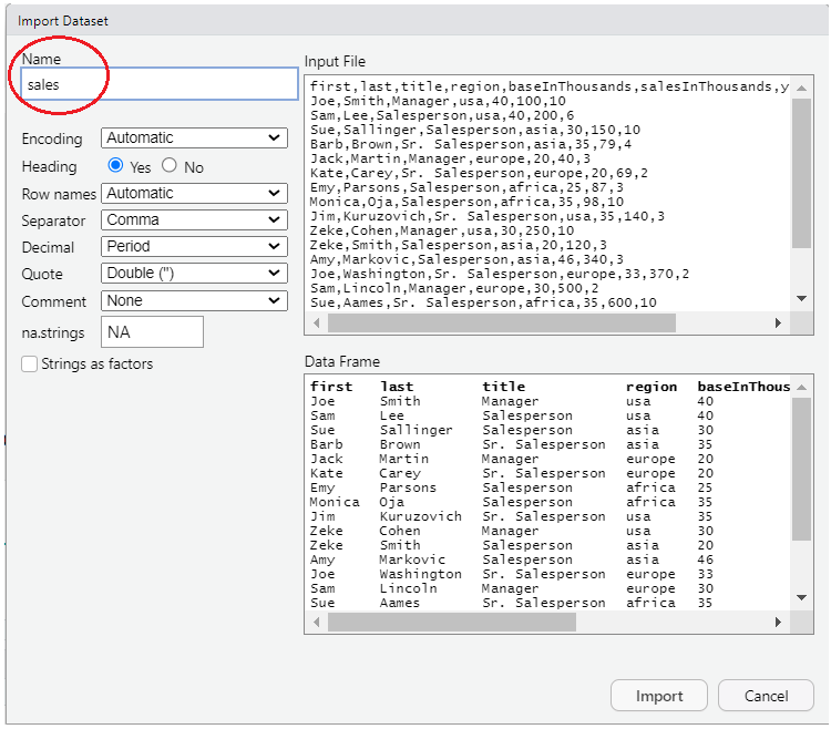
Make sure to change the “Name” portion (see circled section in picture) to read “sales”, then press the “import” button. This will open up a new tab in RStudio that shows the contents of the file. You can safely navigate away from this tab or close the tab and the data will remain imported and can be seen by typing “sales” (without the “quotes”).
12.1.4 Import the data by typing some R code …
The following code reads the data into R. Alternatively, you can follow the instructions above to click on some buttons to import the data.
# Read in the data into a tibble
#
# Note that the following code uses the readr::read_csv function from the readr
# package which is part of the tidyverse collection of packages.
# This function is similar to the base-R read.csv function.
#
# read_csv returns a tibble, which is the data structure that the
# tidyverse packages use in lieu of dataframes. A tibble is basically
# a dataframe with extra features.
# By contrast, the base-r read.csv function returns a dataframe.

sales = read_csv("salespeople-v002.csv", na=c("","NULL"), show_col_types=FALSE)
12.2 Display the data
Since the data is in a tibble, by default, only the first 10 rows are displayed. In addition, only the columns that fit on the screen will be displayed. If the rows are too wide for the screen, then some columns may not be displayed and/or the contents of some columns may be shortened.
# Display the first few rows and columns of the sales data
sales
# A tibble: 24 × 7
first last title region baseInThousands salesInThousands yearsWithCompany
<chr> <chr> <chr> <chr> <dbl> <dbl> <dbl>
1 Joe Smith Mana… usa 40 100 10
2 Sam Lee Sale… usa 40 200 6
3 Sue Sallin… Sale… asia 30 150 10
4 Barb Brown Sr. … asia 35 79 4
5 Jack Martin Mana… europe 20 40 3
6 Kate Carey Sr. … europe 20 69 2
7 Emy Parsons Sale… africa 25 87 3
8 Monica Oja Sale… africa 35 98 10
9 Jim Kuruzo… Sr. … usa 35 140 3
10 Zeke Cohen Mana… usa 30 250 10
# ℹ 14 more rows12.3 Display more rows/columns of the tibble
12.3.1 print( SOME_TIBBLE, n=NUMBER_OF_ROWS)
# Use the print function to modify the output. Use the following arguments:
#    n - number of rows to display (Inf, i.e. infinity, for all rows)
#    width - maximum width of a row to display (might wrap if it's too long for your screen)
print(sales, n=3)
# A tibble: 24 × 7
first last title region baseInThousands salesInThousands yearsWithCompany
<chr> <chr> <chr> <chr> <dbl> <dbl> <dbl>
1 Joe Smith Mana… usa 40 100 10
2 Sam Lee Sale… usa 40 200 6
3 Sue Sallinger Sale… asia 30 150 10
# ℹ 21 more rows12.3.2 print( SOME_TIBBLE, width=WIDTH_OF_DATA)
# Display all rows and all columns
print(sales, n=Inf, width=Inf)
12.3.3 print doesn’t change the tibble
The print function doesn’t change the tibble. print just controls what is displayed to the screen. Therefore if you save the results to a variable, the variable will still contain the entire tibble.
# display first 3 rows
print(sales, n=3)
# A tibble: 24 × 7
first last title region baseInThousands salesInThousands yearsWithCompany
<chr> <chr> <chr> <chr> <dbl> <dbl> <dbl>
1 Joe Smith Mana… usa 40 100 10
2 Sam Lee Sale… usa 40 200 6
3 Sue Sallinger Sale… asia 30 150 10
# ℹ 21 more rows# capture in a variable
x = print(sales, n=3)# A tibble: 24 × 7
first last title region baseInThousands salesInThousands yearsWithCompany
<chr> <chr> <chr> <chr> <dbl> <dbl> <dbl>
1 Joe Smith Mana… usa 40 100 10
2 Sam Lee Sale… usa 40 200 6
3 Sue Sallinger Sale… asia 30 150 10
# ℹ 21 more rows# x still contains ALL the rows
x# A tibble: 24 × 7
first last title region baseInThousands salesInThousands yearsWithCompany
<chr> <chr> <chr> <chr> <dbl> <dbl> <dbl>
1 Joe Smith Mana… usa 40 100 10
2 Sam Lee Sale… usa 40 200 6
3 Sue Sallin… Sale… asia 30 150 10
4 Barb Brown Sr. … asia 35 79 4
5 Jack Martin Mana… europe 20 40 3
6 Kate Carey Sr. … europe 20 69 2
7 Emy Parsons Sale… africa 25 87 3
8 Monica Oja Sale… africa 35 98 10
9 Jim Kuruzo… Sr. … usa 35 140 3
10 Zeke Cohen Mana… usa 30 250 10
# ℹ 14 more rows12.3.4 slice_head, slice_tail, slice_sample, etc
Among some of the many functions included in dplyr are the various “slice_…” functions. These include
- slice - choose rows by row numbers
- slice_head - choose the first n rows (similar to base-R head function)
- slice_tail - choose the last n rows (similar to base-R tail function)
- slice_max - choose the rows with the largest values
- slice_min - choose the rows with the smallest values
- slice_sample - randomly choose a few rows
These functions return a new tibble with just the specified rows that can be saved in a variable. This is different from how the print function works (see above).
See some examples below. See the R documentation for specifics about the various forms of the slice_… functions.
# select just first 3 rows
sales |> slice_head(n=3)
# A tibble: 3 × 7
first last title region baseInThousands salesInThousands yearsWithCompany
<chr> <chr> <chr> <chr> <dbl> <dbl> <dbl>
1 Joe Smith Mana… usa 40 100 10
2 Sam Lee Sale… usa 40 200 6
3 Sue Sallinger Sale… asia 30 150 10# save that in a variable
x = sales |> slice_head(n=3)
# x only contains 3 rows
x# A tibble: 3 × 7
first last title region baseInThousands salesInThousands yearsWithCompany
<chr> <chr> <chr> <chr> <dbl> <dbl> <dbl>
1 Joe Smith Mana… usa 40 100 10
2 Sam Lee Sale… usa 40 200 6
3 Sue Sallinger Sale… asia 30 150 10# print appears to do the same thing
# but print only affects what is displayed to the screen, not
# what is "returned" and can be saved in a variable.
y = sales |> print(n=3)# A tibble: 24 × 7
first last title region baseInThousands salesInThousands yearsWithCompany
<chr> <chr> <chr> <chr> <dbl> <dbl> <dbl>
1 Joe Smith Mana… usa 40 100 10
2 Sam Lee Sale… usa 40 200 6
3 Sue Sallinger Sale… asia 30 150 10
# ℹ 21 more rows# y still has all of the rows
y# A tibble: 24 × 7
first last title region baseInThousands salesInThousands yearsWithCompany
<chr> <chr> <chr> <chr> <dbl> <dbl> <dbl>
1 Joe Smith Mana… usa 40 100 10
2 Sam Lee Sale… usa 40 200 6
3 Sue Sallin… Sale… asia 30 150 10
4 Barb Brown Sr. … asia 35 79 4
5 Jack Martin Mana… europe 20 40 3
6 Kate Carey Sr. … europe 20 69 2
7 Emy Parsons Sale… africa 25 87 3
8 Monica Oja Sale… africa 35 98 10
9 Jim Kuruzo… Sr. … usa 35 140 3
10 Zeke Cohen Mana… usa 30 250 10
# ℹ 14 more rows12.3.5 Other ways of viewing the data
# To see the entire tibble in a separate tab in RStudio
# you can use the following command
#
#View(sales)

# Show all column names and datatypes plus some actual data
glimpse(sales)

# Show just the column names (could be useful for a quick reminder when you need it)
colnames(sales)
12.4 Convert between tibbles and dataframes
The majority of the dplyr functions work with tibbles or dataframes. However, the tidyverse in general and dplyr specifically is designed to work better with tibbles.
If you need to, you can always convert a tibble to a dataframe or a dataframe to a tibble.
# Convert the tibble to a data.frame
dfSales = as.data.frame(sales)

# Convert a dataframe to a tibble
tblSales = as_tibble(dfSales)

# A tibble is also a dataframe.
# This is similar to how a square is also a rectangle.
# You can see that from the class of the variable.
# The class of a tibble contains "tbl_df" "tbl" as well as "data.frame"
class(tblSales)
[1] "tbl_df" "tbl" "data.frame"# However, a dataframe is not necessarily a tibble.
# This is similar ot how a rectangle is not necessarily a square.
# Notice how the class of dfSales is only "data.frame"
class(dfSales)[1] "data.frame"# The head function is designed to work with dataframes
head(dfSales, 3) first last title region baseInThousands salesInThousands
1 Joe Smith Manager usa 40 100
2 Sam Lee Salesperson usa 40 200
3 Sue Sallinger Salesperson asia 30 150
yearsWithCompany
1 10
2 6
3 10# Therefore the head function also works with tibbles
head(tblSales, 3)# A tibble: 3 × 7
first last title region baseInThousands salesInThousands yearsWithCompany
<chr> <chr> <chr> <chr> <dbl> <dbl> <dbl>
1 Joe Smith Mana… usa 40 100 10
2 Sam Lee Sale… usa 40 200 6
3 Sue Sallinger Sale… asia 30 150 10#######################################################################
# However, features of some functions that are designed to
# work with tibbles might not work with data.frames.
######################################################################## This works fine - display the first 3 rows of the tibble.
print(tblSales, n=3) # A tibble: 24 × 7
first last title region baseInThousands salesInThousands yearsWithCompany
<chr> <chr> <chr> <chr> <dbl> <dbl> <dbl>
1 Joe Smith Mana… usa 40 100 10
2 Sam Lee Sale… usa 40 200 6
3 Sue Sallinger Sale… asia 30 150 10
# ℹ 21 more rows# ERROR - n argument is not designed to work with dataframes that aren't tibbles
print(dfSales, n=3) Error in print.default(m, ..., quote = quote, right = right, max = max): invalid 'na.print' specification12.5 select
Use the select function to get just the specified columns.
The first argument to the select function is named .data (notice the period before .data). It is used to specify which tibble or dataframe you are working with. The other arguments are used to specify which columns you’d like to see from the dataframe/tibble. Note that there are NO quotes around the column names (this differs from the base-r way of specifying column names in a dataframe).
# Show just the specified columns from the sales tibble
select(.data=sales, first, last, salesInThousands)
# A tibble: 24 × 3
first last salesInThousands
<chr> <chr> <dbl>
1 Joe Smith 100
2 Sam Lee 200
3 Sue Sallinger 150
4 Barb Brown 79
5 Jack Martin 40
6 Kate Carey 69
7 Emy Parsons 87
8 Monica Oja 98
9 Jim Kuruzovich 140
10 Zeke Cohen 250
# ℹ 14 more rowsThe columns appear in whatever order you specified in the select function. If you want to bring a few columns to the front followed by the rest of the columns, you can use the everything() function.
# Show the specified columns first, followed by the other columns.
select(.data=sales, first, last, everything())
# A tibble: 24 × 7
first last title region baseInThousands salesInThousands yearsWithCompany
<chr> <chr> <chr> <chr> <dbl> <dbl> <dbl>
1 Joe Smith Mana… usa 40 100 10
2 Sam Lee Sale… usa 40 200 6
3 Sue Sallin… Sale… asia 30 150 10
4 Barb Brown Sr. … asia 35 79 4
5 Jack Martin Mana… europe 20 40 3
6 Kate Carey Sr. … europe 20 69 2
7 Emy Parsons Sale… africa 25 87 3
8 Monica Oja Sale… africa 35 98 10
9 Jim Kuruzo… Sr. … usa 35 140 3
10 Zeke Cohen Mana… usa 30 250 10
# ℹ 14 more rows12.6 filter
The filter function is used to retrieve the rows from a tibble that match a condition.
The first argument of the filter function is also .data. Just as with the select function this argument for the filter function is expected to be a tibble or a dataframe.
The next argument to filter is a logical expression. You can use the names of the columns of the tibble/dataframe in the expression. filter will examine each row of the tibble/dataframe and only return those rows whose values match the stated condition.
The following code displays only those rows whose salesInThousands is less than 100.
filter(.data=sales, salesInThousands < 100)# A tibble: 5 × 7
first last title region baseInThousands salesInThousands yearsWithCompany
<chr> <chr> <chr> <chr> <dbl> <dbl> <dbl>
1 Barb Brown Sr. S… asia 35 79 4
2 Jack Martin Manag… europe 20 40 3
3 Kate Carey Sr. S… europe 20 69 2
4 Emy Parsons Sales… africa 25 87 3
5 Monica Oja Sales… africa 35 98 1012.7 Using the dplyr functions in a “pipeline”
The tidyverse functions are designed so that you can be apply them one after the other. The clearest way to do that is to “pipe” the output of one function into the input of another.
The following pipeline first applies select to generate a new tibble that only contains the specified columns. Then the filter function then chooses only those rows that meet the specified condition.
sales |>
  select(first, last, salesInThousands) |>
  filter(salesInThousands < 100)
# A tibble: 5 × 3
first last salesInThousands
<chr> <chr> <dbl>
1 Barb Brown 79
2 Jack Martin 40
3 Kate Carey 69
4 Emy Parsons 87
5 Monica Oja 98# In this example we could apply the filter before select.
# It technically doesn't matter which order you apply the functions in
# as long as you realize that the output of one function is fed into
# the input of the next function.
sales |>
filter(salesInThousands < 100) |>
select(first, last, salesInThousands) # A tibble: 5 × 3
first last salesInThousands
<chr> <chr> <dbl>
1 Barb Brown 79
2 Jack Martin 40
3 Kate Carey 69
4 Emy Parsons 87
5 Monica Oja 98# You can save the results in a variable as follows
lowSales =
sales |>
filter(salesInThousands < 100) |>
select(first, last, salesInThousands)
# Now the lowSales variable contains the results
lowSales# A tibble: 5 × 3
first last salesInThousands
<chr> <chr> <dbl>
1 Barb Brown 79
2 Jack Martin 40
3 Kate Carey 69
4 Emy Parsons 87
5 Monica Oja 98# You can continue to use the new variable for further processing
lowSales |> filter(salesInThousands > 80)# A tibble: 2 × 3
first last salesInThousands
<chr> <chr> <dbl>
1 Emy Parsons 87
2 Monica Oja 9812.8 Important dplyr functions for manipulating tibbles
The dplyr package contains many different functions. The following are the basic dplyr functions that can be used to work with the data in a single tibble or dataframe.
You can combine calls to these functions to retrieve data from a tibble in many different ways. The documentation sometimes refers to these functions as “dplyr verbs” since each of them “do something” to the data. More details about these functions are covered in the sections below.
These dplyr functions all take a tibble as their first argument and return a modified tibble. Therefore each of these functions can be called as part of
a pipeline (see previous section). This allows us to start with some raw data in a tibble and manipulate it in numerous ways.
select - choose the columns you want (this was described above)
filter - choose the rows based on a condition (also described above)
arrange - reorder the rows based on the specified sorting rules
mutate - add additional columns to the tibble/dataframe
group_by - identify which rows will be aggregated by a subsequent call to the summarize function (see below) Note that group_by isn’t too useful unless it is followed by a subsequent call to summarize.
summarize - aggregrate several rows of data into a single row of data by using “aggregate functions” such as max(), min(), etc
There are many other functions included with dplyr. For a full list of what’s included with dplyr run help(package="dplyr"). You can also download a “cheat sheet” that lists all the funcitons at https://www.rstudio.org/links/data_transformation_cheat_sheet (this cheat sheet and others are available from the “Help > Cheat Sheets” menu in RStudio)
12.9 arrange
The arrange function reorders the rows based on specified sorting rules.
# Arrange all of the rows based on salesInThousands.
sales |>
  arrange(salesInThousands)
# A tibble: 24 × 7
first last title region baseInThousands salesInThousands yearsWithCompany
<chr> <chr> <chr> <chr> <dbl> <dbl> <dbl>
1 Jack Martin Mana… europe 20 40 3
2 Kate Carey Sr. … europe 20 69 2
3 Barb Brown Sr. … asia 35 79 4
4 Emy Parsons Sale… africa 25 87 3
5 Monica Oja Sale… africa 35 98 10
6 Joe Smith Mana… usa 40 100 10
7 Jack Aames Sale… usa 43 105 4
8 Larry Green Sr. … europe 20 113 4
9 Zeke Smith Sale… asia 20 120 3
10 Jim Kuruzo… Sr. … usa 35 140 3
# ℹ 14 more rows# Select the first, last names and salesInThousands
# for only those rows for which salesInThousands is less than 100.
# Arrange the rows so that they appear in order of the salesInThousands.
sales |>
select(first, last, salesInThousands) |>
filter(salesInThousands < 100) |>
arrange(salesInThousands)# A tibble: 5 × 3
first last salesInThousands
<chr> <chr> <dbl>
1 Jack Martin 40
2 Kate Carey 69
3 Barb Brown 79
4 Emy Parsons 87
5 Monica Oja 9812.9.1 arrange by more than one column
If you pass more than one column name to the arrange function
the rows are arranged by the first specified column
all rows that have the same value of the first column passed to arrange are further arranged within that cluster of rows by the 2nd column name that was passed to arrange
You can specify as many column names as you like in the arrange function. Column names that appear later in the call to arrange only effect the final order for those rows that share the same value for the earlier column names in the arrange function.
See the examples below.
# show the rows in alphabetical order based on the names of the salespeople.
sales |>
  arrange(last,first) |>
  print(n=Inf)
# A tibble: 24 × 7
first last title region baseInThousands salesInThousands yearsWithCompany
<chr> <chr> <chr> <chr> <dbl> <dbl> <dbl>
1 Barb Aames Sale… usa 21 255 7
2 Jack Aames Sale… usa 43 105 4
3 Sue Aames Sr. … africa 35 600 10
4 Hugh Black Sr. … africa 40 261 9
5 Barb Brown Sr. … asia 35 79 4
6 Jim Brown Sale… europe 50 167 2
7 Kate Carey Sr. … europe 20 69 2
8 Zeke Cohen Mana… usa 30 250 10
9 Larry Green Sr. … europe 20 113 4
10 Jim Kuruzo… Sr. … usa 35 140 3
11 Sam Lee Sale… usa 40 200 6
12 Sam Lincoln Mana… europe 30 500 2
13 Amy Markov… Sale… asia 46 340 3
14 Jack Martin Mana… europe 20 40 3
15 Monica Oja Sale… africa 35 98 10
16 Emy Parsons Sale… africa 25 87 3
17 Sue Sallin… Sale… asia 30 150 10
18 Joe Smith Mana… usa 40 100 10
19 Zeke Smith Sale… asia 20 120 3
20 Joe Washin… Sr. … europe 33 370 2
21 Laura White Mana… africa 20 281 8
22 Emy Zeitch… Mana… asia 34 166 4
23 Kate Zeitch… Sr. … usa 50 187 4
24 Monica Zeitch… Sale… asia 23 184 1# Arrange by title, then by last names and finally by first names
sales |>
arrange(title, last, first) |>
print(n=Inf)# A tibble: 24 × 7
first last title region baseInThousands salesInThousands yearsWithCompany
<chr> <chr> <chr> <chr> <dbl> <dbl> <dbl>
1 Zeke Cohen Mana… usa 30 250 10
2 Sam Lincoln Mana… europe 30 500 2
3 Jack Martin Mana… europe 20 40 3
4 Joe Smith Mana… usa 40 100 10
5 Laura White Mana… africa 20 281 8
6 Emy Zeitch… Mana… asia 34 166 4
7 Barb Aames Sale… usa 21 255 7
8 Jack Aames Sale… usa 43 105 4
9 Jim Brown Sale… europe 50 167 2
10 Sam Lee Sale… usa 40 200 6
11 Amy Markov… Sale… asia 46 340 3
12 Monica Oja Sale… africa 35 98 10
13 Emy Parsons Sale… africa 25 87 3
14 Sue Sallin… Sale… asia 30 150 10
15 Zeke Smith Sale… asia 20 120 3
16 Monica Zeitch… Sale… asia 23 184 1
17 Sue Aames Sr. … africa 35 600 10
18 Hugh Black Sr. … africa 40 261 9
19 Barb Brown Sr. … asia 35 79 4
20 Kate Carey Sr. … europe 20 69 2
21 Larry Green Sr. … europe 20 113 4
22 Jim Kuruzo… Sr. … usa 35 140 3
23 Joe Washin… Sr. … europe 33 370 2
24 Kate Zeitch… Sr. … usa 50 187 4# It might help to read if you display the columns you are sorting by first.
# To do so, simply add a select to the pipeline.
#
# In this example, it makes no difference
# if the select appears before or after the arrange function.
#
# Notice that the names are alphabetically arranged only with a group of
# rows that all have the same title.
sales |>
select(title, last, first, everything()) |>
arrange(title, last, first) |>
print(n=Inf)# A tibble: 24 × 7
title last first region baseInThousands salesInThousands yearsWithCompany
<chr> <chr> <chr> <chr> <dbl> <dbl> <dbl>
1 Manager Cohen Zeke usa 30 250 10
2 Manager Linc… Sam europe 30 500 2
3 Manager Mart… Jack europe 20 40 3
4 Manager Smith Joe usa 40 100 10
5 Manager White Laura africa 20 281 8
6 Manager Zeit… Emy asia 34 166 4
7 Salespe… Aames Barb usa 21 255 7
8 Salespe… Aames Jack usa 43 105 4
9 Salespe… Brown Jim europe 50 167 2
10 Salespe… Lee Sam usa 40 200 6
11 Salespe… Mark… Amy asia 46 340 3
12 Salespe… Oja Moni… africa 35 98 10
13 Salespe… Pars… Emy africa 25 87 3
14 Salespe… Sall… Sue asia 30 150 10
15 Salespe… Smith Zeke asia 20 120 3
16 Salespe… Zeit… Moni… asia 23 184 1
17 Sr. Sal… Aames Sue africa 35 600 10
18 Sr. Sal… Black Hugh africa 40 261 9
19 Sr. Sal… Brown Barb asia 35 79 4
20 Sr. Sal… Carey Kate europe 20 69 2
21 Sr. Sal… Green Larry europe 20 113 4
22 Sr. Sal… Kuru… Jim usa 35 140 3
23 Sr. Sal… Wash… Joe europe 33 370 2
24 Sr. Sal… Zeit… Kate usa 50 187 4# We can get even more fine grained. This time we will arrange
# by title, then by region, then by last names and finally by first names.
#
# Notice that the names are alphabetically arranged only with a group of
# rows that all have the same title and region.
sales |>
select(title, region, last, first, everything()) |>
arrange(title, region, last, first) |>
print(n=Inf)# A tibble: 24 × 7
title region last first baseInThousands salesInThousands yearsWithCompany
<chr> <chr> <chr> <chr> <dbl> <dbl> <dbl>
1 Manager africa White Laura 20 281 8
2 Manager asia Zeit… Emy 34 166 4
3 Manager europe Linc… Sam 30 500 2
4 Manager europe Mart… Jack 20 40 3
5 Manager usa Cohen Zeke 30 250 10
6 Manager usa Smith Joe 40 100 10
7 Salespe… africa Oja Moni… 35 98 10
8 Salespe… africa Pars… Emy 25 87 3
9 Salespe… asia Mark… Amy 46 340 3
10 Salespe… asia Sall… Sue 30 150 10
11 Salespe… asia Smith Zeke 20 120 3
12 Salespe… asia Zeit… Moni… 23 184 1
13 Salespe… europe Brown Jim 50 167 2
14 Salespe… usa Aames Barb 21 255 7
15 Salespe… usa Aames Jack 43 105 4
16 Salespe… usa Lee Sam 40 200 6
17 Sr. Sal… africa Aames Sue 35 600 10
18 Sr. Sal… africa Black Hugh 40 261 9
19 Sr. Sal… asia Brown Barb 35 79 4
20 Sr. Sal… europe Carey Kate 20 69 2
21 Sr. Sal… europe Green Larry 20 113 4
22 Sr. Sal… europe Wash… Joe 33 370 2
23 Sr. Sal… usa Kuru… Jim 35 140 3
24 Sr. Sal… usa Zeit… Kate 50 187 412.9.2 desc(SOME_COLUMN) - arrange in descending order
Use the desc function to specify “descending” order. See the examples.
# In the following, the rows with the highest values
# of salesInThousands are at the top.

sales |>
  filter(salesInThousands < 100) |>
  select(first, last, salesInThousands) |>
  arrange(desc(salesInThousands))  |>
  print(n=Inf)
# A tibble: 5 × 3
first last salesInThousands
<chr> <chr> <dbl>
1 Monica Oja 98
2 Emy Parsons 87
3 Barb Brown 79
4 Kate Carey 69
5 Jack Martin 40# Arrange alphabetically by the region.
# Within each region, show the sales in decreasing order.
sales |>
select(region, baseInThousands, everything()) |>
arrange(region, desc(baseInThousands)) |>
print(n=Inf)# A tibble: 24 × 7
region baseInThousands first last title salesInThousands yearsWithCompany
<chr> <dbl> <chr> <chr> <chr> <dbl> <dbl>
1 africa 40 Hugh Black Sr. … 261 9
2 africa 35 Monica Oja Sale… 98 10
3 africa 35 Sue Aames Sr. … 600 10
4 africa 25 Emy Parsons Sale… 87 3
5 africa 20 Laura White Mana… 281 8
6 asia 46 Amy Markov… Sale… 340 3
7 asia 35 Barb Brown Sr. … 79 4
8 asia 34 Emy Zeitch… Mana… 166 4
9 asia 30 Sue Sallin… Sale… 150 10
10 asia 23 Monica Zeitch… Sale… 184 1
11 asia 20 Zeke Smith Sale… 120 3
12 europe 50 Jim Brown Sale… 167 2
13 europe 33 Joe Washin… Sr. … 370 2
14 europe 30 Sam Lincoln Mana… 500 2
15 europe 20 Jack Martin Mana… 40 3
16 europe 20 Kate Carey Sr. … 69 2
17 europe 20 Larry Green Sr. … 113 4
18 usa 50 Kate Zeitch… Sr. … 187 4
19 usa 43 Jack Aames Sale… 105 4
20 usa 40 Joe Smith Mana… 100 10
21 usa 40 Sam Lee Sale… 200 6
22 usa 35 Jim Kuruzo… Sr. … 140 3
23 usa 30 Zeke Cohen Mana… 250 10
24 usa 21 Barb Aames Sale… 255 7# Show the names, titles and salesInThousands for
# people who sell to the usa and for people who sell to europe.
#
# Arrange the results so that all titles are grouped together.
# Within the rows of a particular title sort the results in
# descending order based on the salesInThousands so that the
# rows with greater salesInThousands appear earlier.
#
# Only show salespeople for the usa and europe
sales |>
select(first, last, title, salesInThousands, region) |>
filter(region %in% c("usa", "europe")) |>
arrange(title, desc(salesInThousands))# A tibble: 13 × 5
first last title salesInThousands region
<chr> <chr> <chr> <dbl> <chr>
1 Sam Lincoln Manager 500 europe
2 Zeke Cohen Manager 250 usa
3 Joe Smith Manager 100 usa
4 Jack Martin Manager 40 europe
5 Barb Aames Salesperson 255 usa
6 Sam Lee Salesperson 200 usa
7 Jim Brown Salesperson 167 europe
8 Jack Aames Salesperson 105 usa
9 Joe Washington Sr. Salesperson 370 europe
10 Kate Zeitchik Sr. Salesperson 187 usa
11 Jim Kuruzovich Sr. Salesperson 140 usa
12 Larry Green Sr. Salesperson 113 europe
13 Kate Carey Sr. Salesperson 69 europe# Careful - if you do not include region in the select , it won't work
# ERROR - object 'region' not found
sales |>
select(first, last, title, salesInThousands) |> # region is missing here
filter(region %in% c("usa", "europe")) |> # but you need it here
arrange(title, desc(salesInThousands))Error in `filter()`:
ℹ In argument: `region %in% c("usa", "europe")`.
Caused by error:
! object 'region' not found# Rearrange the order of the function calls to get it to work
sales |>
arrange(title, desc(salesInThousands)) |>
filter(region %in% c("usa", "europe")) |> # we use region here
select(first, last, title, salesInThousands) # we can now exclude region# A tibble: 13 × 4
first last title salesInThousands
<chr> <chr> <chr> <dbl>
1 Sam Lincoln Manager 500
2 Zeke Cohen Manager 250
3 Joe Smith Manager 100
4 Jack Martin Manager 40
5 Barb Aames Salesperson 255
6 Sam Lee Salesperson 200
7 Jim Brown Salesperson 167
8 Jack Aames Salesperson 105
9 Joe Washington Sr. Salesperson 370
10 Kate Zeitchik Sr. Salesperson 187
11 Jim Kuruzovich Sr. Salesperson 140
12 Larry Green Sr. Salesperson 113
13 Kate Carey Sr. Salesperson 6912.10 mutate - add new columns
Use the mutate function to add new columns. These new columns can be based on existing data. See the examples below.
# All salespeople get a commission equal to 10% of their sales.
# Create a new column with the name commission that shows the value of their commission.

# The following code creates the new column as the last column in the tibble.
sales |>
  mutate(commission=0.10*salesInThousands, takeHome=baseInThousands + 0.10*salesInThousands ) |>
  print(width=Inf)
# A tibble: 24 × 9
first last title region baseInThousands salesInThousands
<chr> <chr> <chr> <chr> <dbl> <dbl>
1 Joe Smith Manager usa 40 100
2 Sam Lee Salesperson usa 40 200
3 Sue Sallinger Salesperson asia 30 150
4 Barb Brown Sr. Salesperson asia 35 79
5 Jack Martin Manager europe 20 40
6 Kate Carey Sr. Salesperson europe 20 69
7 Emy Parsons Salesperson africa 25 87
8 Monica Oja Salesperson africa 35 98
9 Jim Kuruzovich Sr. Salesperson usa 35 140
10 Zeke Cohen Manager usa 30 250
yearsWithCompany commission takeHome
<dbl> <dbl> <dbl>
1 10 10 50
2 6 20 60
3 10 15 45
4 4 7.9 42.9
5 3 4 24
6 2 6.9 26.9
7 3 8.7 33.7
8 10 9.8 44.8
9 3 14 49
10 10 25 55
# ℹ 14 more rows12.10.1 .before and .after
Use the .before and .after argument to mutate to specify where the new columns should appear in the tibble. See the examples below.
# Place the newly created column at the beginning of the tibble,
# i.e. .before the 1st column.

sales |>
  mutate(commission=0.10*salesInThousands, .before=1)
# A tibble: 24 × 8
commission first last title region baseInThousands salesInThousands
<dbl> <chr> <chr> <chr> <chr> <dbl> <dbl>
1 10 Joe Smith Manager usa 40 100
2 20 Sam Lee Salespe… usa 40 200
3 15 Sue Sallinger Salespe… asia 30 150
4 7.9 Barb Brown Sr. Sal… asia 35 79
5 4 Jack Martin Manager europe 20 40
6 6.9 Kate Carey Sr. Sal… europe 20 69
7 8.7 Emy Parsons Salespe… africa 25 87
8 9.8 Monica Oja Salespe… africa 35 98
9 14 Jim Kuruzovich Sr. Sal… usa 35 140
10 25 Zeke Cohen Manager usa 30 250
# ℹ 14 more rows
# ℹ 1 more variable: yearsWithCompany <dbl># Place the newly created column as the 3rd column
# i.e. .after the 2nd column.
# (.before=4 would also work)
sales |>
mutate(commission=0.10*salesInThousands, .after=2)# A tibble: 24 × 8
first last commission title region baseInThousands salesInThousands
<chr> <chr> <dbl> <chr> <chr> <dbl> <dbl>
1 Joe Smith 10 Manager usa 40 100
2 Sam Lee 20 Salespe… usa 40 200
3 Sue Sallinger 15 Salespe… asia 30 150
4 Barb Brown 7.9 Sr. Sal… asia 35 79
5 Jack Martin 4 Manager europe 20 40
6 Kate Carey 6.9 Sr. Sal… europe 20 69
7 Emy Parsons 8.7 Salespe… africa 25 87
8 Monica Oja 9.8 Salespe… africa 35 98
9 Jim Kuruzovich 14 Sr. Sal… usa 35 140
10 Zeke Cohen 25 Manager usa 30 250
# ℹ 14 more rows
# ℹ 1 more variable: yearsWithCompany <dbl># .before and .after can also refer to specific columns
# For example the following also places the commission after the last name column
sales |>
mutate(commission=0.10*salesInThousands, .after=last)# A tibble: 24 × 8
first last commission title region baseInThousands salesInThousands
<chr> <chr> <dbl> <chr> <chr> <dbl> <dbl>
1 Joe Smith 10 Manager usa 40 100
2 Sam Lee 20 Salespe… usa 40 200
3 Sue Sallinger 15 Salespe… asia 30 150
4 Barb Brown 7.9 Sr. Sal… asia 35 79
5 Jack Martin 4 Manager europe 20 40
6 Kate Carey 6.9 Sr. Sal… europe 20 69
7 Emy Parsons 8.7 Salespe… africa 25 87
8 Monica Oja 9.8 Salespe… africa 35 98
9 Jim Kuruzovich 14 Sr. Sal… usa 35 140
10 Zeke Cohen 25 Manager usa 30 250
# ℹ 14 more rows
# ℹ 1 more variable: yearsWithCompany <dbl>12.10.2 a new column that depends on other new columns
The following code creates two new columns.
The commission column is created as in the last example.
The takeHome column is the total take home pay for the salesperson, i.e. their baseInThousands plus the commission.
If you create both columns in a single call to mutate, you will need to repeat the calculation for the commission twice (see examples below). An alternative is to call the mutate function twice. For tibbles with many rows this can take longer to process but is less error prone when you write the code.
# All salespeople get a commission equal to 10% of their sales.
# Create a new column with the name commission that shows the value of their commission.
# Create another column called takeHome which has their total takehome pay.

# We can do it all in one call to mutate.
# However, that require repeating the code for calculating for the commission.
sales |>
  mutate(commission=0.10*salesInThousands, takeHome=baseInThousands + 0.10*salesInThousands, .before=1 ) |>
  print(width=Inf)
# A tibble: 24 × 9
commission takeHome first last title region baseInThousands
<dbl> <dbl> <chr> <chr> <chr> <chr> <dbl>
1 10 50 Joe Smith Manager usa 40
2 20 60 Sam Lee Salesperson usa 40
3 15 45 Sue Sallinger Salesperson asia 30
4 7.9 42.9 Barb Brown Sr. Salesperson asia 35
5 4 24 Jack Martin Manager europe 20
6 6.9 26.9 Kate Carey Sr. Salesperson europe 20
7 8.7 33.7 Emy Parsons Salesperson africa 25
8 9.8 44.8 Monica Oja Salesperson africa 35
9 14 49 Jim Kuruzovich Sr. Salesperson usa 35
10 25 55 Zeke Cohen Manager usa 30
salesInThousands yearsWithCompany
<dbl> <dbl>
1 100 10
2 200 6
3 150 10
4 79 4
5 40 3
6 69 2
7 87 3
8 98 10
9 140 3
10 250 10
# ℹ 14 more rows# By separating the code into two calls to mutate, we can refer to the
# newly created "commission" column when calculating the takeHome column.
# Note that the 2nd call to mutate below receives a tibble that already has a
# commission column as the first column. That is why .before=2 (and not .before=1)
sales |>
mutate(commission=0.10*salesInThousands, .before=1) |>
mutate(takeHome=baseInThousands + commission, .before=2) |>
print(width=Inf)# A tibble: 24 × 9
commission takeHome first last title region baseInThousands
<dbl> <dbl> <chr> <chr> <chr> <chr> <dbl>
1 10 50 Joe Smith Manager usa 40
2 20 60 Sam Lee Salesperson usa 40
3 15 45 Sue Sallinger Salesperson asia 30
4 7.9 42.9 Barb Brown Sr. Salesperson asia 35
5 4 24 Jack Martin Manager europe 20
6 6.9 26.9 Kate Carey Sr. Salesperson europe 20
7 8.7 33.7 Emy Parsons Salesperson africa 25
8 9.8 44.8 Monica Oja Salesperson africa 35
9 14 49 Jim Kuruzovich Sr. Salesperson usa 35
10 25 55 Zeke Cohen Manager usa 30
salesInThousands yearsWithCompany
<dbl> <dbl>
1 100 10
2 200 6
3 150 10
4 79 4
5 40 3
6 69 2
7 87 3
8 98 10
9 140 3
10 250 10
# ℹ 14 more rows12.11 distinct()
The distinct function eliminates any duplicate rows from a tibble. See the examples.
# Show the just the region for each row in the tibble
sales |>
  select (region) |>
  print(n=Inf)
# A tibble: 24 × 1
region
<chr>
1 usa
2 usa
3 asia
4 asia
5 europe
6 europe
7 africa
8 africa
9 usa
10 usa
11 asia
12 asia
13 europe
14 europe
15 africa
16 usa
17 usa
18 usa
19 asia
20 asia
21 europe
22 europe
23 africa
24 africa# Same thing using distinct()
# Show just the distinct (ie. different) regions
sales |>
select (region) |>
distinct() |> # show just the distinct rows
print(n=Inf)# A tibble: 4 × 1
region
<chr>
1 usa
2 asia
3 europe
4 africa###############################################################
# NOTE - all values in the row must be exactly the same
# for the distinct() function to eliminate the duplicate rows.
###############################################################
# Show the region and title for rows
# whose region is either europe or asia.
# Arrange the output so they come up sorted.
sales |>
select(region, title) |>
filter(region %in% c('europe', 'asia')) |>
arrange(region, title) |>
print(n=Inf)# A tibble: 12 × 2
region title
<chr> <chr>
1 asia Manager
2 asia Salesperson
3 asia Salesperson
4 asia Salesperson
5 asia Salesperson
6 asia Sr. Salesperson
7 europe Manager
8 europe Manager
9 europe Salesperson
10 europe Sr. Salesperson
11 europe Sr. Salesperson
12 europe Sr. Salesperson# Same thing using distinct()
# Show just the distinct rows from the previous command
sales |>
select(region, title) |>
filter(region %in% c('europe', 'asia')) |>
distinct() |> # eliminate duplicate rows
arrange(region, title) |>
print(n=Inf)# A tibble: 6 × 2
region title
<chr> <chr>
1 asia Manager
2 asia Salesperson
3 asia Sr. Salesperson
4 europe Manager
5 europe Salesperson
6 europe Sr. Salesperson# Notice that in the previous output, there were multiple
# rows that contained "europe", multiple rows that contained "asia"
# as well as multiple rows that contained each of the different titles.
# However - there were NO rows that contained exact duplicates of both
# the region and the title.
#
# The moral of the story is that distinct() will only elminate rows
# that are EXACT duplicates in EVERY column.sales |>
select(region, title, everything()) |>
arrange(region, title)# A tibble: 24 × 7
region title first last baseInThousands salesInThousands yearsWithCompany
<chr> <chr> <chr> <chr> <dbl> <dbl> <dbl>
1 africa Manager Laura White 20 281 8
2 africa Salespe… Emy Pars… 25 87 3
3 africa Salespe… Moni… Oja 35 98 10
4 africa Sr. Sal… Sue Aames 35 600 10
5 africa Sr. Sal… Hugh Black 40 261 9
6 asia Manager Emy Zeit… 34 166 4
7 asia Salespe… Sue Sall… 30 150 10
8 asia Salespe… Zeke Smith 20 120 3
9 asia Salespe… Amy Mark… 46 340 3
10 asia Salespe… Moni… Zeit… 23 184 1
# ℹ 14 more rowssales |>
select(region, title) |>
arrange(region, title)# A tibble: 24 × 2
region title
<chr> <chr>
1 africa Manager
2 africa Salesperson
3 africa Salesperson
4 africa Sr. Salesperson
5 africa Sr. Salesperson
6 asia Manager
7 asia Salesperson
8 asia Salesperson
9 asia Salesperson
10 asia Salesperson
# ℹ 14 more rowssales |>
select(region,title) |>
arrange(region, title) |>
distinct()# A tibble: 12 × 2
region title
<chr> <chr>
1 africa Manager
2 africa Salesperson
3 africa Sr. Salesperson
4 asia Manager
5 asia Salesperson
6 asia Sr. Salesperson
7 europe Manager
8 europe Salesperson
9 europe Sr. Salesperson
10 usa Manager
11 usa Salesperson
12 usa Sr. Salesperson12.12 summarize and group_by
The summarize() and group_by() functions work together. We’ll explain exactly how below …
12.12.1 aggregate functions
The summarize function is used to condense the contents of several rows of data into a single row of data. It does this by using functions such as min(), max(), mean(), etc. These functions can take several values and return a single value. Such functions are known as aggregate functions.
12.12.2 summarize (without group_by)
The summarize function is often preceded by a call to the group_by() function (which we will cover in the next section). group_by() is used to contol which rows of data will be affected by a subsequent call to the summarize() function. This will be explained in more detail below. For now, we will just focus on how summarize() works when it is NOT preceded by a call to group_by().
When summarize() is NOT preceded by a call to group_by() then the job of the summarize() function is to return a single row of summary by applying aggregate functions (such as min, max, mean, etc) to columns of the tibble.
See the examples below.
# mean salesInThousands (for all rows)
# Note that this returns a tibble with exactly one row and one column.
sales |>
summarize(mean(salesInThousands))# A tibble: 1 × 1
`mean(salesInThousands)`
<dbl>
1 203.# We can change the column name as shown below
sales |>
summarize(averageSales = mean(salesInThousands))# A tibble: 1 × 1
averageSales
<dbl>
1 203.# We can filter the rows before calculating the mean results (or use any other of the dplyr functions)
#
# Show the mean sales for just the USA.
sales |>
filter(region == "usa") |>
summarize(usaSales = mean(salesInThousands))# A tibble: 1 × 1
usaSales
<dbl>
1 177.# We can get more than one column in our summary tibble
sales |>
summarize(meanSales = mean(salesInThousands), maxSales=max(salesInThousands), minSales=min(salesInThousands),
maxBase = max(baseInThousands), minBase=min(baseInThousands))# A tibble: 1 × 5
meanSales maxSales minSales maxBase minBase
<dbl> <dbl> <dbl> <dbl> <dbl>
1 203. 600 40 50 2012.12.3 The n() function
The n() function returns the number of rows.
The n_distinct() function returns the number of rows that have distinct (i.e. different) values.
# Show all of the rows ordered by region and title
sales |>
select(region, title, everything()) |>
print(n=Inf)# A tibble: 24 × 7
region title first last baseInThousands salesInThousands yearsWithCompany
<chr> <chr> <chr> <chr> <dbl> <dbl> <dbl>
1 usa Manager Joe Smith 40 100 10
2 usa Salespe… Sam Lee 40 200 6
3 asia Salespe… Sue Sall… 30 150 10
4 asia Sr. Sal… Barb Brown 35 79 4
5 europe Manager Jack Mart… 20 40 3
6 europe Sr. Sal… Kate Carey 20 69 2
7 africa Salespe… Emy Pars… 25 87 3
8 africa Salespe… Moni… Oja 35 98 10
9 usa Sr. Sal… Jim Kuru… 35 140 3
10 usa Manager Zeke Cohen 30 250 10
11 asia Salespe… Zeke Smith 20 120 3
12 asia Salespe… Amy Mark… 46 340 3
13 europe Sr. Sal… Joe Wash… 33 370 2
14 europe Manager Sam Linc… 30 500 2
15 africa Sr. Sal… Sue Aames 35 600 10
16 usa Salespe… Barb Aames 21 255 7
17 usa Salespe… Jack Aames 43 105 4
18 usa Sr. Sal… Kate Zeit… 50 187 4
19 asia Manager Emy Zeit… 34 166 4
20 asia Salespe… Moni… Zeit… 23 184 1
21 europe Salespe… Jim Brown 50 167 2
22 europe Sr. Sal… Larry Green 20 113 4
23 africa Manager Laura White 20 281 8
24 africa Sr. Sal… Hugh Black 40 261 9# n() - returns the number of rows in the tibble
# n_distinct(COL1, COL2, ...) - returns the number of rows for which
# the specified columns taken all together are distinct among all other rows.
sales |>
select(region, title, everything()) |>
summarize(n(), n_distinct(region), n_distinct(title), n_distinct(region, title))# A tibble: 1 × 4
`n()` `n_distinct(region)` `n_distinct(title)` `n_distinct(region, title)`
<int> <int> <int> <int>
1 24 4 3 1212.13 group_by and summarize (or summarise)
The examples above for summarize all return a single row of data. This is because they are summarizing all of the rows for the tibble that summarize received. Note that this is true even if the rows have been filtered first. For example:
# The following returns just one row.
# The summarize function is summarizing ALL of the rows
# for the tibble that it was given.
sales %>%
filter(region == "usa") |>
summarize(numberOfRows=n(), maxUsaSales = max(salesInThousands), minUsaSales=min(salesInThousands))# A tibble: 1 × 3
numberOfRows maxUsaSales minUsaSales
<int> <dbl> <dbl>
1 7 255 100The functions, group_by and summarize functions are designed to work together. The job of the group_by function is to separate the rows of data into different “groups” that will later be processed separately by the summarize function.
If you use a group_by function in general it is followed a call to summarize()
To understand the examples below, it is helpful to first see the rows sorted by region and title
sales |>
  select(region, title, everything()) |>
  arrange(region, title)
# A tibble: 24 × 7
region title first last baseInThousands salesInThousands yearsWithCompany
<chr> <chr> <chr> <chr> <dbl> <dbl> <dbl>
1 africa Manager Laura White 20 281 8
2 africa Salespe… Emy Pars… 25 87 3
3 africa Salespe… Moni… Oja 35 98 10
4 africa Sr. Sal… Sue Aames 35 600 10
5 africa Sr. Sal… Hugh Black 40 261 9
6 asia Manager Emy Zeit… 34 166 4
7 asia Salespe… Sue Sall… 30 150 10
8 asia Salespe… Zeke Smith 20 120 3
9 asia Salespe… Amy Mark… 46 340 3
10 asia Salespe… Moni… Zeit… 23 184 1
# ℹ 14 more rowsNotice how the rows that have the same region can be thought of as a “group” of rows for that region.
See the examples below
# Show summary information for each of the different regions.
# Each row in the output corresponds only to the rows for the region shown on that row of output.
sales |>
  group_by(region) |>    # create a different group for each region
  summarize(numberOfRows=n(), mean(baseInThousands), mean(salesInThousands))
# A tibble: 4 × 4
region numberOfRows `mean(baseInThousands)` `mean(salesInThousands)`
<chr> <int> <dbl> <dbl>
1 africa 5 31 265.
2 asia 6 31.3 173.
3 europe 6 28.8 210.
4 usa 7 37 177.Similarly we can group the rows by those with the same value in the title column.
# Show summary information for each of the different titles.
# Each row in the output corresponds only to the rows for the title shown on that row of output.
sales |>
  group_by(title) |>    # create a different group for each title
  summarize(numberOfRows=n(), mean(baseInThousands), mean(salesInThousands))
# A tibble: 3 × 4
title numberOfRows `mean(baseInThousands)` `mean(salesInThousands)`
<chr> <int> <dbl> <dbl>
1 Manager 6 29 223.
2 Salesperson 10 33.3 171.
3 Sr. Salesperson 8 33.5 227.12.13.1 group_by without summarize has no noticeable effect
Note that on its own, the group_by function doesn’t appear to do anything. It only has a tangible effect when a summarize function is called after the group_by function
# group_by without a subsequent call to summarize doesn't appear to do anything special
sales |>
  group_by(title)
# A tibble: 24 × 7
# Groups: title [3]
first last title region baseInThousands salesInThousands yearsWithCompany
<chr> <chr> <chr> <chr> <dbl> <dbl> <dbl>
1 Joe Smith Mana… usa 40 100 10
2 Sam Lee Sale… usa 40 200 6
3 Sue Sallin… Sale… asia 30 150 10
4 Barb Brown Sr. … asia 35 79 4
5 Jack Martin Mana… europe 20 40 3
6 Kate Carey Sr. … europe 20 69 2
7 Emy Parsons Sale… africa 25 87 3
8 Monica Oja Sale… africa 35 98 10
9 Jim Kuruzo… Sr. … usa 35 140 3
10 Zeke Cohen Mana… usa 30 250 10
# ℹ 14 more rows12.13.2 group_by more than one column
A call to group_by that has more than one column creates a separate group for the rows that have the same values for all of the specified columns. To understand this look at the following output:
asia_europe_sales =
  sales |>
    select(region, title, baseInThousands) |>
    filter(region %in% c('europe', 'asia')) |>
    arrange(region, title)

asia_europe_sales  |>
    print(n=Inf)
# A tibble: 12 × 3
region title baseInThousands
<chr> <chr> <dbl>
1 asia Manager 34
2 asia Salesperson 30
3 asia Salesperson 20
4 asia Salesperson 46
5 asia Salesperson 23
6 asia Sr. Salesperson 35
7 europe Manager 20
8 europe Manager 30
9 europe Salesperson 50
10 europe Sr. Salesperson 20
11 europe Sr. Salesperson 33
12 europe Sr. Salesperson 20We can treat the rows that have the same values for both the region and title as a single group of rows. For example we can treat all of the rows for “asia Salesperson” as a group and the rows for “eroupe Manager” as a separate group. The output of the following command returns one row for each group.
# create groups based on region and sales
asia_europe_sales |>
  group_by(region, title) |>
  summarize(n(), max(baseInThousands), mean(baseInThousands))|>
  print(n=Inf)
`summarise()` has grouped output by 'region'. You can override using the
`.groups` argument.# A tibble: 6 × 5
# Groups: region [2]
region title `n()` `max(baseInThousands)` `mean(baseInThousands)`
<chr> <chr> <int> <dbl> <dbl>
1 asia Manager 1 34 34
2 asia Salesperson 4 46 29.8
3 asia Sr. Salesperson 1 35 35
4 europe Manager 2 30 25
5 europe Salesperson 1 50 50
6 europe Sr. Salesperson 3 33 24.3
Note
You might be wondering about the somewhat cryptic message from the previous command:
summarise()has grouped output by ‘region’. You can override using the.groupsargument.
When group_by is called with more than one column name the subsequent summarize call will generate a message similar to the one shown above. You can ignore this message without any issue. If you want to understand it better - look at this.
12.13.3 order of columns in group_by is irrelevant
Note that it makes no difference which order you specify the column names in the call to group by. The following command reverses the order of the columns in the call to group_by but returns the exact same result as the previous command.
# create groups based on region and sales
asia_europe_sales |>
  group_by(title, region) |>   # the order of the columns in group_by makes no difference
  summarize(n(), max(baseInThousands), mean(baseInThousands))|>
  print(n=Inf)
`summarise()` has grouped output by 'title'. You can override using the
`.groups` argument.# A tibble: 6 × 5
# Groups: title [3]
title region `n()` `max(baseInThousands)` `mean(baseInThousands)`
<chr> <chr> <int> <dbl> <dbl>
1 Manager asia 1 34 34
2 Manager europe 2 30 25
3 Salesperson asia 4 46 29.8
4 Salesperson europe 1 50 50
5 Sr. Salesperson asia 1 35 35
6 Sr. Salesperson europe 3 33 24.312.13.4 some other aggregate functions
As mentioned above, an “aggregate function” is a function that can take several values as input but returns a single value. It is these types of functions that are used by summarize()
The following are some other commonly used aggregate functions that can be used in summarize. There are many, many others.
Statistics: mean(), median(), sd(), IQR(), mad()
Range: min(), max(),
Position: first(), last(), nth(),
Counting: n(), n_distinct()
Logical: any(), all()