if(!require(tibble)){install.packages("tibble");require(tibble);}
if(!require(dplyr)){install.packages("dplyr");require(dplyr);}
if(!require(readr)){install.packages("readr");require(readr);}
if(!require(sqldf)){install.packages("sqldf");require(sqldf);}13 SQL Select
13.1 NOTE - this page is for “IDS2040 - Data Management” (not “IDS1020 - Intro to IDS”)
NOTE - If you are in my “IDS1020 - Intro to IDS” class, this is NOT the page you should be reading. Rather, jump to the next section entitled “Relational Databases and SQL” and start from there.
This page is intended for my “IDS460 - Data Management” class. The info below assumes that you have some knowledge of the dplyr package in R (which was covered in the previous section). After you get a basic idea of what the SQL SELECT statement does and how it is very similar to the dplyr functions, you can move onto the next section entitled “Relational Databases and SQL” and continue with that information.
13.2 Get the data
The data we are using in this section contains information about salespeople who are employees of a company. Each row of the data contains info about one salesperson. The salespeople get paid some “base pay” as well as a commission that is a percent of the total dollar amount of sales they make.
Follow the instructions below to get the data and start using it in R.
13.2.1 Load the R packages we’ll neeed
13.2.2 Download the file
The data is contained in a csv file. If you’d like to follow along with this tutorial on your own computer you can download the .csv file we are using by clicking here.
13.2.3 Import the data by clicking on some buttons …
The code in the next section below uses read_csv function to read the data into R. If you are not comfortable with R, I recommend that you instead, follow the instructions starting in the next bullet to import the data into R.
If you are not familiar with R, you may have some trouble running the read_csv() code shown below. Instead, I recommend that you follow the following instructions to import the file into R.
To do so, click on “Import Dataset” button on the “Environment” tab (usually found in the upper-right-hand window pane in RStudio).
Choose “From Text (base)” and locate your file. You should see something like this:
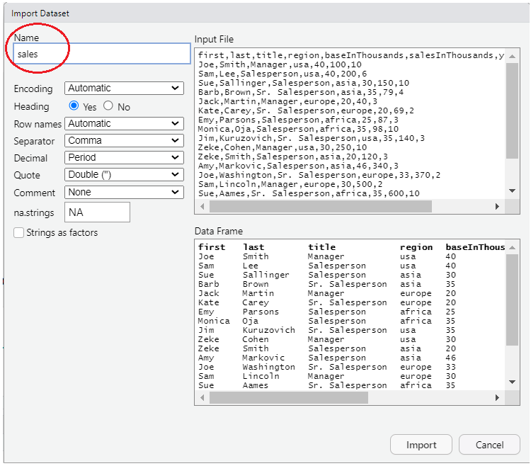
Make sure to change the “Name” portion (see circled section in picture) to read “sales”, then press the “import” button. This will open up a new tab in RStudio that shows the contents of the file. You can safely navigate away from this tab or close the tab and the data will remain imported and can be seen by typing “sales” (without the “quotes”).
13.2.4 Import the data by typing some R code …
The following code reads the data into R. Alternatively, you can follow the instructions above to click on some buttons to import the data.
# Read in the data into a tibble
#
# Note that the following code uses the readr::read_csv function from the readr
# package which is part of the tidyverse collection of packages.
# This function is similar to the base-R read.csv function.
#
# read_csv returns a tibble, which is the data structure that the
# tidyverse packages use in lieu of dataframes. A tibble is basically
# a dataframe with extra features.
# By contrast, the base-r read.csv function returns a dataframe.

sales = read_csv("salespeople-v002.csv", na=c("","NULL"), show_col_types=FALSE)
13.3 Databases and SQL
A database is an organized collection of data that is designed to be accessed and manipulated by computer programs. We’ll cover a little more about exactly what a database is and how it differs from Excel, R and other programs in the next section of this book. Below is just a brief explanation to give you some background before we start getting into the details of the SQL language that is used to communicate with databases.
A “relational database” is a type of database in which data is arranged in “tables” that are organized into “rows” and “columns”. A “relational database table” is very similar to an R dataframe or tibble. Relational databases are controlled and managed with software known as “Relational DataBase Management System” (RDBMS) software. Relational database technology dates back to the 1970s and has been around long before R has been around. Relational databases are used by just about every major company all around the world.
“Structured Query Language” (or SQL for short - pronounced “sequel”) is the standard language that is used to communicate with a DBMS to manage and manipulate the data in a Relational Database. SQL has many different commands. One of the most important SQL commands for data analysts to know is the SQL “SELECT” command. It is this command that is used to extract data from a database and organize the data into a desired form. We will focus in this section on an intro to the SQL SELECT statement.
As we said above, R is NOT a Database Management System. However SQL is a very popular language. Many technologists come to R, already having a deep knowledge of the SQL language. Therefore it is nice to know that the SQL language can also be used to manipulate R dataframes. This is possible because R dataframes are very, very similar in structure to Relational Database “tables” (i.e. they have rows, columns, column names and specific datatypes for each column).
The R “sqldf” package includes a function named “sqldf” which takes a SQL command as its argument. Wherever the SQL command refers to the name of a relational database “table”, sqldf runs the SQL command using the R dataframe with that name.
13.4 dplyr is very similar to the SQL SELECT command
The designers of dplyr got inspiration for many of their ideas from SQL. Therefore once you know the basics of dplyr it should be very easy to transfer that knowledge to learning the SQL SELECT statement.
The following examples show how the concepts you learned in the previous section about dplyr carry over to the SQL SELECT statement.
The English word “query” means a question. A SQL SELECT statement is often referred to as a database “query”. In essence a SQL SELECT statement in essence asks the database a question and gets back an answer.
13.5 SQL SELECT “clauses” compared with dplyr “functions”
While dplyr uses different “functions”, the SQL SELECT statement is comprised of different “clauses”. The clauses in the SQL SELECT statement are listed below. We will elaborate on the details of these clauses in the sections below.
SELECT
This is used to “select” the columns you want - similar to dplyr select function.
FROM
Used to specify which “tables” contain the information you will be working with. In dplyr this is accomplished via the first argument, .data, of each of the dplyr “verb” functions that we learned about in the previous section.
WHERE
Choose the rows you want. Directly analogous to the dplyr “filter” function.
GROUP BY
Directly analogous to the dplyr “group_by” function.
HAVING
This is also similar to the dplyr “filter” function. We will learn later how this differs from the SQL SELECT WHERE clause.
ORDER BY
Directly analogous to the dplyr “arrange” function
LIMIT
Directly analogous to the dplyr print(n=…) function or the dplyr slice_head(n=…) function.
13.6 Order of the clauses is important
A SQL SELECT statement may contain some or all of the above clauses. Only the SELECT clause is absolutely required. If the SQL SELECT statement contains more than one clause then whichever clauses do appear must appear in the order listed above.
13.7 Is SQL case sensitive? yes and no
Different SQL products treat case sensitivity differently. In general the names of tables and columns ARE case sensitive. The “keywords” of the language are generally NOT case sensitive. However, it is often the convention of many SQL books and references to show SQL keywords in UPPER CASE. We have done that below but it is not strictly necessary.
13.8 Whitespace in SQL commands is ignored
A SQL command may be written entirely on one line. However, extra whitespace (i.e. spaces, tabs, newlines) may be added to make the code more readable. It is common to start each SQL SELECT statement clause on a new line and to add extra whitespace to make the code more readable. In general we tried to follow that practice in the code.
13.9 Intro to ERDs - i.e. “Entity Relationship Diagrams”
An “Entity Relationship Diagram” (ERD) is a diagram that highlights the structure of the tables in a database (in database terminology tables are also known as “entity sets” or “entity types” - see below). The ERD does NOT show the data in the tables, just the structure of the tables. The following is an ERD for the sales data we have been using.
Note that so far we’ve only been using one table. An ERD gets more complicated when a database contains several tables. We will revisit ERDs again later.
erDiagram
    SALES {
        first character "employee first name"
        last character "employee last name"
        title character "employee title"
        region character "region that employee sells to"
        baseInThousands numeric "employee's base pay (in thousands)"
        salesInThousands numeric "total sales dollars (in thousands)"
        yearsWithCompany numeric "number years employee with company"
    }
- The table name is shown at the top
- Under the table name
- The 1st column contains the names of the table’s fields (i.e. columns)
- The 2nd column contains the datatype of the fields
- The 3rd column contains a description of the field
Some Entity Relationship Diagrams don’t contain as much information. Often an ERD will NOT contain a description of the fields. This is still a “valid” ERD, just not as descriptive.
erDiagram
    SALES {
        first character
        last character
        title character
        region character
        baseInThousands numeric
        salesInThousands numeric
        yearsWithCompany numeric
    }
In the extreme case, an ERD may only contain the names of the tables. This type of ERD is only really useful when the database contains multiple tables.
erDiagram
    SALES
13.10 Database terminology - fields, entities, etc
There are different terms used to refer to the rows and columns of a table, dataframe or tibble. Statisticians often refer to each row of a table as an observation and each column of a table as a variable.
In the world of databases, a column can be referred to as a “column” or a “field”. Rows are referred to as just “rows” but sometimes are referred to as “records” or “entities”. Often an entire table is referred to as an “entity” (technically a table, which is a collection of rows, is an “entity set” or an “entity type”).
The truth is not many people use the word “entity” or “entity set”. However, an “Entity Relationship Diagram” is used to show the tables in a database and how the tables are “related” to each other.
In this section we are just focusing on a single table. In a later sections, we’ll learn more about “relationships” between multiple tables and how the relationships are displayed on an Entity Relationship Diagram.
13.11 SELECT and FROM clauses
# The SELECT clause specifies which columns you want.
# The FROM clause specifies the table (or tables) that contain the data.
sqldf("SELECT title, first, last
       FROM sales")
title first last
1 Manager Joe Smith
2 Salesperson Sam Lee
3 Salesperson Sue Sallinger
4 Sr. Salesperson Barb Brown
5 Manager Jack Martin
6 Sr. Salesperson Kate Carey
7 Salesperson Emy Parsons
8 Salesperson Monica Oja
9 Sr. Salesperson Jim Kuruzovich
10 Manager Zeke Cohen
11 Salesperson Zeke Smith
12 Salesperson Amy Markovic
13 Sr. Salesperson Joe Washington
14 Manager Sam Lincoln
15 Sr. Salesperson Sue Aames
16 Salesperson Barb Aames
17 Salesperson Jack Aames
18 Sr. Salesperson Kate Zeitchik
19 Manager Emy Zeitchik
20 Salesperson Monica Zeitchik
21 Salesperson Jim Brown
22 Sr. Salesperson Larry Green
23 Manager Laura White
24 Sr. Salesperson Hugh Black# SELECT * in SQL is similar to select(everything()) in dplyr.
# * is an abbreviation for all of the column names.
sqldf("SELECT *
FROM sales") first last title region baseInThousands salesInThousands yearsWithCompany
1 Joe Smith Manager usa 40 100 10
2 Sam Lee Salesperson usa 40 200 6
3 Sue Sallinger Salesperson asia 30 150 10
4 Barb Brown Sr. Salesperson asia 35 79 4
5 Jack Martin Manager europe 20 40 3
6 Kate Carey Sr. Salesperson europe 20 69 2
7 Emy Parsons Salesperson africa 25 87 3
8 Monica Oja Salesperson africa 35 98 10
9 Jim Kuruzovich Sr. Salesperson usa 35 140 3
10 Zeke Cohen Manager usa 30 250 10
11 Zeke Smith Salesperson asia 20 120 3
12 Amy Markovic Salesperson asia 46 340 3
13 Joe Washington Sr. Salesperson europe 33 370 2
14 Sam Lincoln Manager europe 30 500 2
15 Sue Aames Sr. Salesperson africa 35 600 10
16 Barb Aames Salesperson usa 21 255 7
17 Jack Aames Salesperson usa 43 105 4
18 Kate Zeitchik Sr. Salesperson usa 50 187 4
19 Emy Zeitchik Manager asia 34 166 4
20 Monica Zeitchik Salesperson asia 23 184 1
21 Jim Brown Salesperson europe 50 167 2
22 Larry Green Sr. Salesperson europe 20 113 4
23 Laura White Manager africa 20 281 8
24 Hugh Black Sr. Salesperson africa 40 261 9# Unfortunately, the SQL SELECT * is not as smart as the everything() function in dplyr.
# In dplyr, everything() does not include columns that you already typed.
# In SQL, the * always includes ALL columns. Therefore the following
# query displays the title and region columns a 2nd time due to the *
sqldf("SELECT title, region, *
FROM sales") title region first last title region baseInThousands salesInThousands yearsWithCompany
1 Manager usa Joe Smith Manager usa 40 100 10
2 Salesperson usa Sam Lee Salesperson usa 40 200 6
3 Salesperson asia Sue Sallinger Salesperson asia 30 150 10
4 Sr. Salesperson asia Barb Brown Sr. Salesperson asia 35 79 4
5 Manager europe Jack Martin Manager europe 20 40 3
6 Sr. Salesperson europe Kate Carey Sr. Salesperson europe 20 69 2
7 Salesperson africa Emy Parsons Salesperson africa 25 87 3
8 Salesperson africa Monica Oja Salesperson africa 35 98 10
9 Sr. Salesperson usa Jim Kuruzovich Sr. Salesperson usa 35 140 3
10 Manager usa Zeke Cohen Manager usa 30 250 10
11 Salesperson asia Zeke Smith Salesperson asia 20 120 3
12 Salesperson asia Amy Markovic Salesperson asia 46 340 3
13 Sr. Salesperson europe Joe Washington Sr. Salesperson europe 33 370 2
14 Manager europe Sam Lincoln Manager europe 30 500 2
15 Sr. Salesperson africa Sue Aames Sr. Salesperson africa 35 600 10
16 Salesperson usa Barb Aames Salesperson usa 21 255 7
17 Salesperson usa Jack Aames Salesperson usa 43 105 4
18 Sr. Salesperson usa Kate Zeitchik Sr. Salesperson usa 50 187 4
19 Manager asia Emy Zeitchik Manager asia 34 166 4
20 Salesperson asia Monica Zeitchik Salesperson asia 23 184 1
21 Salesperson europe Jim Brown Salesperson europe 50 167 2
22 Sr. Salesperson europe Larry Green Sr. Salesperson europe 20 113 4
23 Manager africa Laura White Manager africa 20 281 8
24 Sr. Salesperson africa Hugh Black Sr. Salesperson africa 40 261 9# The only thing you can do in a select statement without a FROM clause
# is to perform calculations without data from a table.
sqldf("SELECT 3+2, 100*5") 3+2 100*5
1 5 50013.12 add new columns in SELECT clause
# In dplyr, to add new columns you use the mutate function.
# In the SQL SELECT command this is accomplished as part of the SELECT clause.
# To add new columns that are calculated from other columns
# simply add the calculations to the select clause.

sqldf("SELECT first, last, salesInThousands, 0.1 * salesInThousands
       FROM sales
       ")
first last salesInThousands 0.1 * salesInThousands
1 Joe Smith 100 10.0
2 Sam Lee 200 20.0
3 Sue Sallinger 150 15.0
4 Barb Brown 79 7.9
5 Jack Martin 40 4.0
6 Kate Carey 69 6.9
7 Emy Parsons 87 8.7
8 Monica Oja 98 9.8
9 Jim Kuruzovich 140 14.0
10 Zeke Cohen 250 25.0
11 Zeke Smith 120 12.0
12 Amy Markovic 340 34.0
13 Joe Washington 370 37.0
14 Sam Lincoln 500 50.0
15 Sue Aames 600 60.0
16 Barb Aames 255 25.5
17 Jack Aames 105 10.5
18 Kate Zeitchik 187 18.7
19 Emy Zeitchik 166 16.6
20 Monica Zeitchik 184 18.4
21 Jim Brown 167 16.7
22 Larry Green 113 11.3
23 Laura White 281 28.1
24 Hugh Black 261 26.1# You can give the new column a unique name by following the definition
# of the column with "AS columnName".
sqldf("SELECT first, last, salesInThousands, 0.1 * salesInThousands as commission
FROM sales
") first last salesInThousands commission
1 Joe Smith 100 10.0
2 Sam Lee 200 20.0
3 Sue Sallinger 150 15.0
4 Barb Brown 79 7.9
5 Jack Martin 40 4.0
6 Kate Carey 69 6.9
7 Emy Parsons 87 8.7
8 Monica Oja 98 9.8
9 Jim Kuruzovich 140 14.0
10 Zeke Cohen 250 25.0
11 Zeke Smith 120 12.0
12 Amy Markovic 340 34.0
13 Joe Washington 370 37.0
14 Sam Lincoln 500 50.0
15 Sue Aames 600 60.0
16 Barb Aames 255 25.5
17 Jack Aames 105 10.5
18 Kate Zeitchik 187 18.7
19 Emy Zeitchik 166 16.6
20 Monica Zeitchik 184 18.4
21 Jim Brown 167 16.7
22 Larry Green 113 11.3
23 Laura White 281 28.1
24 Hugh Black 261 26.1# The word "AS" is actually optional. The following adds two new columns
# but does not use the word AS. All you need is the definition of the column
# followed by a space followed by the name of the new column.
sqldf("SELECT first, last, baseInThousands,
salesInThousands, 0.1 * salesInThousands commission,
salesInThousands * 0.1 + baseInThousands takeHome
FROM sales
WHERE region='africa'
") first last baseInThousands salesInThousands commission takeHome
1 Emy Parsons 25 87 8.7 33.7
2 Monica Oja 35 98 9.8 44.8
3 Sue Aames 35 600 60.0 95.0
4 Laura White 20 281 28.1 48.1
5 Hugh Black 40 261 26.1 66.113.13 use aggregate functions in SELECT to create summary rows
# The dplyr summarize function is used to summarize (or aggregate) info from
# several rows into a single row.
#
# In the SQL SELECT statement, this is accomplished by simply using
# aggregate functions in the select clause.
#
# SQL has several built in standard aggregate functions
#
#   count(*) - similar to n() in dplyr - we'll discuss why the * is there later
#   avg(SOME_COLUMN)
#   max(SOME_COLUMN)
#   min(SOME_COLUMN)

sqldf("select count(*), avg(baseInThousands), max(baseInThousands)
       FROM sales
       ORDER BY region ASC, salesInThousands DESC")
count(*) avg(baseInThousands) max(baseInThousands)
1 24 32.29167 50# As shown above we can assign names to the new columns.
# Again, the word "AS" is optional. The following statement
# would work exactly the same way if we did not have the word "AS"
sqldf("SELECT count(*) as numberOfEmployees,
avg(baseInThousands) AS averagebaseInThousands,
max(baseInThousands) AS maxbaseInThousands
FROM sales
ORDER BY region ASC, salesInThousands DESC") numberOfEmployees averagebaseInThousands maxbaseInThousands
1 24 32.29167 50# This is the same query as above.
# This version does not have the word "AS".
# The results are exactly the same.
sqldf("SELECT count(*) as numberOfEmployees,
avg(baseInThousands) averagebaseInThousands,
max(baseInThousands) maxbaseInThousands
FROM sales
ORDER BY region ASC, salesInThousands DESC") numberOfEmployees averagebaseInThousands maxbaseInThousands
1 24 32.29167 5013.14 WHERE clause
# WHERE is directly analogous to the dplyr filter function.
#
# The WHERE clause identifies the rows that will be returned.
# It takes a logical expression that uses the names of the columns.
# For every row the SELECT statement analyzes the row and calculates the
# result of the logical expression for that row. If the logical expression
# for a row is TRUE you get the row back. If not you do not get the row.

sqldf("SELECT *
       FROM sales
       WHERE salesInThousands < 100")
first last title region baseInThousands salesInThousands yearsWithCompany
1 Barb Brown Sr. Salesperson asia 35 79 4
2 Jack Martin Manager europe 20 40 3
3 Kate Carey Sr. Salesperson europe 20 69 2
4 Emy Parsons Salesperson africa 25 87 3
5 Monica Oja Salesperson africa 35 98 10# This query uses aggregate functions in the SELECT but does NOT have a WHERE.
# Therefore the result is a summary of ALL rows in the table.
sqldf("SELECT count(*), min(baseInThousands), max(baseInThousands), avg(baseInThousands)
FROM sales") count(*) min(baseInThousands) max(baseInThousands) avg(baseInThousands)
1 24 20 50 32.29167# This is the same query but adds WHERE region='asia'.
# As a result the summary row only reflects info about the rows for 'asia'.
# Notice the there are fewer rows in the count(*) column and some of the
# other summary statistics are also different.
sqldf("SELECT count(*), min(baseInThousands), max(baseInThousands), avg(baseInThousands)
FROM sales
WHERE region='asia'") count(*) min(baseInThousands) max(baseInThousands) avg(baseInThousands)
1 6 20 46 31.3333313.15 ORDER BY clause
# The ORDER BY clause is directly anaogous to dplyr's arrange function

sqldf("SELECT *
       FROM sales
       WHERE salesInThousands < 100
       ORDER By salesInThousands")
first last title region baseInThousands salesInThousands yearsWithCompany
1 Jack Martin Manager europe 20 40 3
2 Kate Carey Sr. Salesperson europe 20 69 2
3 Barb Brown Sr. Salesperson asia 35 79 4
4 Emy Parsons Salesperson africa 25 87 3
5 Monica Oja Salesperson africa 35 98 10# Just as with dplyr's arrange function the rows can be ordered
# from largest to smallest by specifying desc, i.e. a descending order
# for the values of a column.
sqldf("SELECT *
FROM sales
WHERE salesInThousands < 100
ORDER BY salesInThousands DESC") first last title region baseInThousands salesInThousands yearsWithCompany
1 Monica Oja Salesperson africa 35 98 10
2 Emy Parsons Salesperson africa 25 87 3
3 Barb Brown Sr. Salesperson asia 35 79 4
4 Kate Carey Sr. Salesperson europe 20 69 2
5 Jack Martin Manager europe 20 40 3# Just as with dplyr's arrange function you can specify that the order
# of the rows should depend on multiple columns.
#
# The first column specified is used to order all of the rows.
# Subsequent columns mentioned in ORDER By are used only for rows
# in which the values for the earlier columns are the same.
#
# Each column could have an ascending (asc) or descending (desc) order.
# If neither asc nor desc is specified, then the default is an ascending order.
sqldf("SELECT *
FROM sales
ORDER BY region ASC, salesInThousands DESC") first last title region baseInThousands salesInThousands yearsWithCompany
1 Sue Aames Sr. Salesperson africa 35 600 10
2 Laura White Manager africa 20 281 8
3 Hugh Black Sr. Salesperson africa 40 261 9
4 Monica Oja Salesperson africa 35 98 10
5 Emy Parsons Salesperson africa 25 87 3
6 Amy Markovic Salesperson asia 46 340 3
7 Monica Zeitchik Salesperson asia 23 184 1
8 Emy Zeitchik Manager asia 34 166 4
9 Sue Sallinger Salesperson asia 30 150 10
10 Zeke Smith Salesperson asia 20 120 3
11 Barb Brown Sr. Salesperson asia 35 79 4
12 Sam Lincoln Manager europe 30 500 2
13 Joe Washington Sr. Salesperson europe 33 370 2
14 Jim Brown Salesperson europe 50 167 2
15 Larry Green Sr. Salesperson europe 20 113 4
16 Kate Carey Sr. Salesperson europe 20 69 2
17 Jack Martin Manager europe 20 40 3
18 Barb Aames Salesperson usa 21 255 7
19 Zeke Cohen Manager usa 30 250 10
20 Sam Lee Salesperson usa 40 200 6
21 Kate Zeitchik Sr. Salesperson usa 50 187 4
22 Jim Kuruzovich Sr. Salesperson usa 35 140 3
23 Jack Aames Salesperson usa 43 105 4
24 Joe Smith Manager usa 40 100 1013.16 GROUP BY clause
# The GROUP BY clause in SQL is directly analogous to the group_by function in dplyr.
#
# All of the rows that have the same value for the specified GROUP BY columns
# are aggregated (i.e. summarized) in a single line of output.
#
# GROUP BY should only be used if the SELECT clause includes aggregate functions.

sqldf("SELECT title, count(*), avg(baseInThousands) avgBase, max(baseInThousands) maxBase
       FROM sales
       GROUP BY title
       ORDER BY title")
title count(*) avgBase maxBase
1 Manager 6 29.0 40
2 Salesperson 10 33.3 50
3 Sr. Salesperson 8 33.5 50# Grouping by a different column - region
sqldf("SELECT region, count(*), avg(baseInThousands) avgBase, max(baseInThousands) maxBase
FROM sales
GROUP BY region
ORDER BY region") region count(*) avgBase maxBase
1 africa 5 31.00000 40
2 asia 6 31.33333 46
3 europe 6 28.83333 50
4 usa 7 37.00000 50# Just as with dplyr, the groups can be defined by more than one column.
#
# The following query treats all of the rows that match in both the
# region and title columns as a single group.
#
# For example, all of the original rows from the sales table
# that have a title of "Salesperson" and a region of "asia"
# are considered to be part of the same group and are summarized
# in a single row of the output.
sqldf("SELECT title, region, count(*), avg(baseInThousands) avgBase, max(baseInThousands) maxBase
FROM sales
GROUP BY title, region
ORDER BY title, region") title region count(*) avgBase maxBase
1 Manager africa 1 20.00000 20
2 Manager asia 1 34.00000 34
3 Manager europe 2 25.00000 30
4 Manager usa 2 35.00000 40
5 Salesperson africa 2 30.00000 35
6 Salesperson asia 4 29.75000 46
7 Salesperson europe 1 50.00000 50
8 Salesperson usa 3 34.66667 43
9 Sr. Salesperson africa 2 37.50000 40
10 Sr. Salesperson asia 1 35.00000 35
11 Sr. Salesperson europe 3 24.33333 33
12 Sr. Salesperson usa 2 42.50000 50# A similar query without a GROUP BY returns just a single row that
# summarizes the data from all rows of the table.
sqldf("SELECT count(*), avg(baseInThousands) avgBase, max(baseInThousands) maxBase
FROM sales") count(*) avgBase maxBase
1 24 32.29167 5013.17 LIMIT clause
# The LIMIT clause is similar to print(n=) with dplyr.
# It limits the number of rows returned to the first few
# that would have been returned had the query not included the LIMIT clause.
#
# The LIMIT clause is usually used with an ORDER BY clause.

sqldf("SELECT *
       FROM sales
       ORDER BY salesInThousands desc
       LIMIT 10")
first last title region baseInThousands salesInThousands yearsWithCompany
1 Sue Aames Sr. Salesperson africa 35 600 10
2 Sam Lincoln Manager europe 30 500 2
3 Joe Washington Sr. Salesperson europe 33 370 2
4 Amy Markovic Salesperson asia 46 340 3
5 Laura White Manager africa 20 281 8
6 Hugh Black Sr. Salesperson africa 40 261 9
7 Barb Aames Salesperson usa 21 255 7
8 Zeke Cohen Manager usa 30 250 10
9 Sam Lee Salesperson usa 40 200 6
10 Kate Zeitchik Sr. Salesperson usa 50 187 4# Note that the LIMIT clause is not standard SQL - some SQL flavors
# do not contain a LIMIT clause. However, the LIMIT clause or
# something similar is part of many SQL flavors.