############################################################################################## factors#### For more info see this page:## https://swcarpentry.github.io/r-novice-inflammation/12-supp-factors/index.html####################################################################################################################################################################.# NUMBERS SHOULDN'T ALWAYS BE USED FOR DOING MATH ... ## Some types of numbers are not intended for doing math. For example,# suppose I asked 1000 people: ## Which of the following do you like best: # "chicken" or "pizza" or "pasta"## and I get 1000 answers - that look like this:# "pizza" "chicken" "pizza" "pasta" "chicken" "pizza" ... etc## I can put that data into an R vector# answers = c("pizza","chicken","pizza","pasta","chicken","pizza", etc ...)## but there is not much that I can do with that vector other than figure out# how many answers I got for each type of food, e.g. 300 for "chicken",# 500 for "pizza" and 200 for "pasta". There is no way for me to take# the "mean" of the answers and come up with "pizza flavored chicken"## Similarly, if I changed the question to the following:## Which of the following do you like best:# answer 1 for "chicken" or 2 for "pizza" or 3 for "pasta"## and I get 1000 answers - that look like this:# 2 1 2 3 1 2 ... etc## I can put that data into an R vector# answers = c(2, 1, 2, 3, 1, 2, ... etc)## However, even though the answers now look like numbers taking the mean of # those numbers would not make any sense. (The mean would be meaningless :)# 1, 2 and 3 are simply standing in for the values "chicken" "pizza" and "pasta".# Taking a mean of these numbers would make no more sense than taking a# mean of c("pizza","chicken","pizza", etc ...).## So we can see clearly that you shouldn't always do "math" with numbers.########################################################################.#########################################################################.# SOME CHARACTER DATA IS NOT INTENDED FOR TALLYING RESULTS## For some character data it is appropriate to add up how many copies of # the same value appear in the data. In the example above in response to# asking 1000 people the question:# which do you like best "chicken" "pizza" or "pasta"## we might put the results in a character vector, e.g.# answers = c("pizza","chicken","pizza","pasta","chicken","pizza", etc ...)## It would be very appropriate to "tally these values" (ie. add up how many# of each response there is). For example we might figure out there were# 300 answers for "chicken", 500 for "pizza" and 200 for "pasta".### However, suppose I have data in parallel vectors that record info about# students in a school. The vectors might look like this:# studentNames = c("Mike Smith", "Anne Jones", "Larry Cohen", ... etc)# year = c("sophomore", "freshman", "sophomore", ... etc)# age = c(18, 21, 16, ... etc)# satMath = c(400, 650, 520, ... etc)## A statistician working with the data to figure out school policy and# demographics would typically not need to tally# the student names, e.g. 1 "Mike Smith", 1 "Anne Jones", 1 "Larry Cohen", etc.## NOTE - it might be interesting to know if there are two people with the # same name - HOWEVER - a "statistician working with the data to figure out# school policy and demographics" would not need to do that. ###########################################################################.###########################################################################.## *** INTRODUCING R "factors" ***## DIFFERENT TYPES OF NUMBERS ... DIFFERENT TYPES OF CHARACTERS ...# = DIFFERENT "classes" OF DATA IN R### As we know R has the following "classes" of data that are intended to be used# in the following ways:## "numeric" vectors - for numbers for which doing "math" is appropriate## "character" vectors - for data that has no inherent meaning and does # NOT need to be tallied (e.g. studentNames in example above)## R also has another class of data:## "factor" vectors - used for numeric data that is NOT appropriate for math# also used for character data that is not appropriate for tallying## For example you could use an R "factor" to store the answers# to either question about favorite food, whether the # answers are given with words, e.g. "pizza", "chicken" , etc# or if the answers are given with numbers, e.g. # 1 for chicken, 2 for pizza, etc.## KEEP READING FOR MORE INFO ABOUT HOW TO WORK WITH FACTORS IN R############################################################################.#------------------------------------------------------------------------------# Different types of data in statistics# See this for a good overview:## https://www.scribbr.com/statistics/levels-of-measurement/#:~:text=Nominal%3A%20the%20data%20can%20only%20be%20categorized.,and%20has%20a%20natural%20zero.### - nominal/categorical data ## (ratios are OK, > and < are not OK, means are not OK)# R uses "factor", i.e. factor( ... ) - see below#### - ordinal data (ratios are OK, > and < are OK, means are not OK) # R uses "ordered factor", ie. factor( ..., ordered=TRUE)#### - interval data (see the above webpage)# - ratio data (ratios are OK, > and < are OK, means are OK) ## R uses "numeric" for both of these types of data# (also "integer" and "double" - these are beyond the scope of what we've discussed)#------------------------------------------------------------------------------#------------------------------------------------------------------------------# What is a factor? ## A "factor" is R's way of making it easy for statisticians to work with# nominal/categorical data.## A factor ...# - is a vector# - has a "class" attribute that is set to "factor"# - has a "levels" attribute that contains a vector of level names# (see more below)#------------------------------------------------------------------------------# character data - is used for data that is not going to be involved in statistical calculations# # Data such as peoples names are generally not used for statistical analysis.# For example, I generally wouldn't care about what the most common name is# in my data or what percent of the people have each name or what the ratio# is of "joes" to "bobs" in my data. These are all questions that don't really# make any difference to a typical statistician.# The name of the person is simply a name that I can use to refer to the data for that person.## Character data that you are not expecting to use for statistical analysis should# simply remain as "character" data - NOT as a factor.## [ If for some reason you DO care about statistical analysis of the names of the# people then you could make this data into a factor. ]person <-c("joe", "sue", "bob", "alan", "anne", "pearl") person
[1] "joe" "sue" "bob" "alan" "anne" "pearl"
class(person) # "character"
[1] "character"
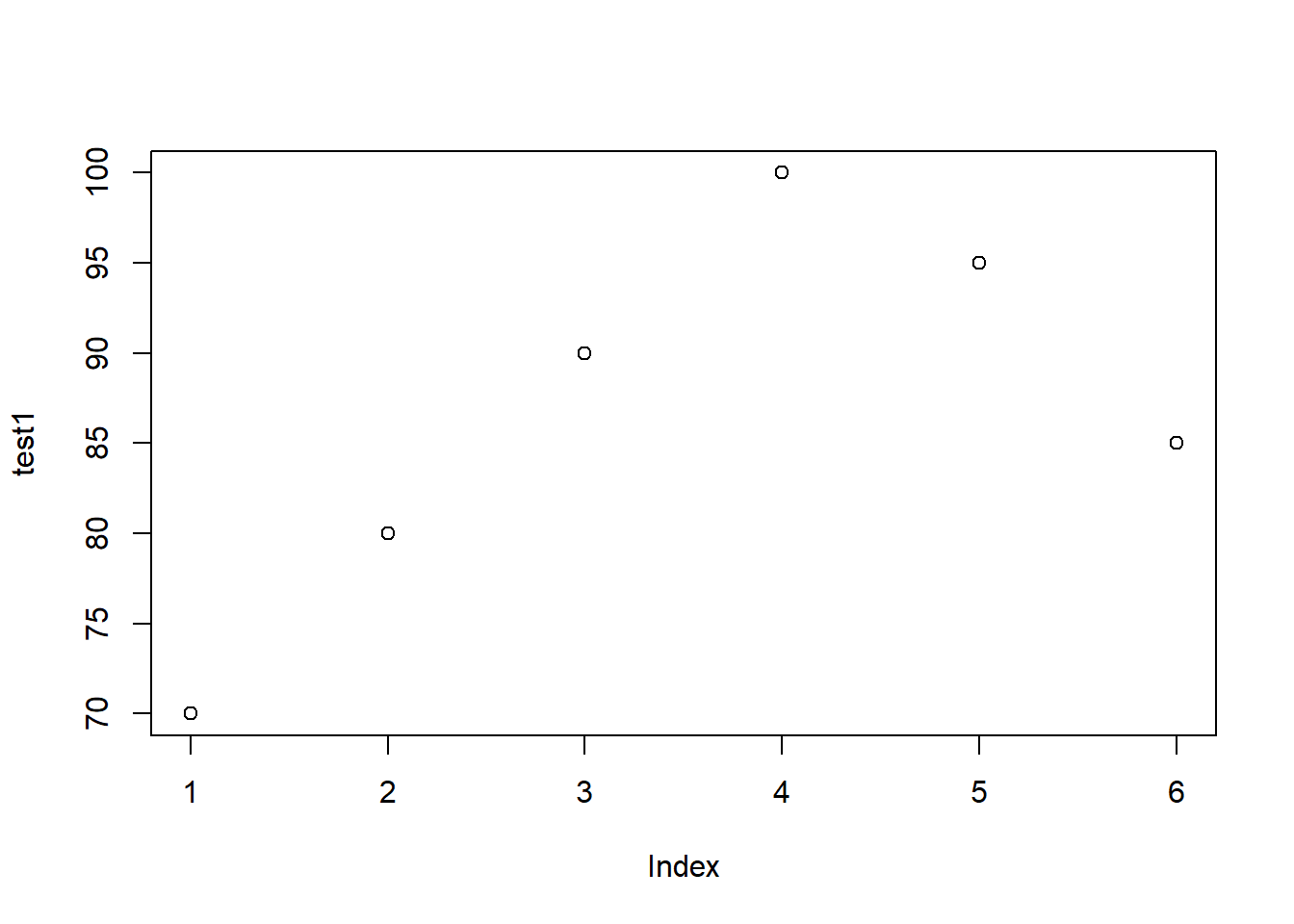
# numeric data is data for which you expect to perform mathematical operations# such as: + - * / ^ sqrt, max, min, sum, mean, etc.# This type of data should NOT be made into a factor.## For example test grades that will be analyzed numerically - eg. mean, max, etc# should NOT be a factor.test1 <-c(70,80,90,100,95,85) test1
[1] 70 80 90 100 95 85
class(test1) # "numeric"
[1] "numeric"
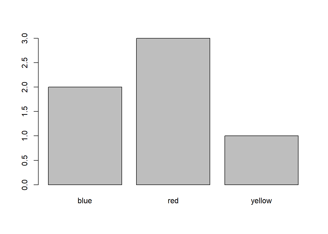
# For nominal/categorical data use a factor in R.## For example, let's say you would want to perform statistical analysis# on people's favorite colors. For example you might be curious to know# how many people have "blue" as their favorite color, what is the most common# favorite color or what percent of the people have each favorite color# then favorite color should be a factor.favcolor <-factor(c("red", "blue", "red", "red", "blue", "yellow")) favcolor
[1] red    blue   red    red    blue   yellow
Levels: blue red yellow
class(favcolor) # "factor"
[1] "factor"
# The "levels" of a factor are the different values that the data can have.# For the favcolors data shown above, the valid values are "red", "blue" and# "yellow". These are the levels of the factor.levels(favcolor) # "blue" "red" "yellow" (in alphabetical order)
[1] "blue" "red" "yellow"
#------------------------------------------------------------------------------# plot( x ) # works differently for different classes of x# summary( x ) # works differently for different classes of x## Some R functions will work differently with factor data than with# other types of data.## Examples: summary, plot#------------------------------------------------------------------------------summary(favcolor) # for factors shows the number of each "level" in the data (see output)
  blue    red yellow
     2      3      1
summary(test1) # for numeric shows a numeric summary (see output)
   Min. 1st Qu.  Median    Mean 3rd Qu.    Max.
  70.00   81.25   87.50   86.67   93.75  100.00
summary(person) # for character not much useful data (see output)
   Length     Class      Mode
        6 character character
plot(favcolor) # a bar chart of the numbers of number of values for each color
plot(test1) # a "dot plot" of the values of each individual test grade
plot(person) # ERROR - you cannot plot character data
Warning in xy.coords(x, y, xlabel, ylabel, log): NAs introduced by coercion
Warning in min(x): no non-missing arguments to min; returning Inf
Warning in max(x): no non-missing arguments to max; returning -Inf
Error in plot.window(...): need finite 'ylim' values
#.............................................................................# WARNING - if you try calling plot from RStudio and the window that displays# the plot is too small to display the plot you may get an error similar to# the following:## > plot(person)# Error in plot.new() : figure margins too large## To fix this, simply make the window for the plot larger and run the command again.#.............................................................................#------------------------------------------------------------------------------# An "ordered factor" is R's way of working with ordinal data.# An ordered factor ...# - ... is a vector# - ... has a "class" attribute that is set to "ordered" factor"# - ... has a "levels" attribute that contains a vector of level names# (see more below)#------------------------------------------------------------------------------# ordinal data (use an "ordered factor" in R)## nominal/categorical data that also have an implied "order" to the data# is known as "ordinal" data and should be stored as an "ordered factor"# # For example, students in college are categorized as freshmen, sophomores,# juniors and seniors. However, there is also an implied order, in that# the category depends on the number of credits taken (or the number of year# in college). Freshmen have the fewest credits (or years in college) # while seniors have the most credits (or years in school). This implies# the order freshman, sophomore, junior, senior.## Notice that I included a "levels" argument in the call to the factor function# to list the exact levels. The values in the levels argument should be# arranged in the correct order.year <-factor(c("fr", "so", "fr", "so", "fr", "se"),ordered=TRUE,levels=c("fr","so","ju","se")) year
[1] fr so fr so fr se
Levels: fr < so < ju < se
class(year) # "ordered" "factor"
[1] "ordered" "factor"
levels(year) # "fr" "so" "ju" "se"
[1] "fr" "so" "ju" "se"
plot(year) # all 4 levels - including ju are plotted# WHAT IF YOU DID NOT SPECIFY levels= ... AND ordered = TRUEyear <-factor(c("fr", "so", "fr", "so", "fr", "se"),ordered=TRUE) year
[1] fr so fr so fr se
Levels: fr < se < so
class(year) # "ordered" "factor"
[1] "ordered" "factor"
levels(year) # "fr" "se" "so" - "ju" isn't there - the order is alphabetical
[1] "fr" "se" "so"
plot(year) # no column for ju and columns are in alphabetical order# WHAT IF YOU DID NOT SPECIFY levels= ... AND ordered = FALSE year <-factor(c("fr", "so", "fr", "so", "fr", "se"),ordered=FALSE) year
[1] fr so fr so fr se
Levels: fr se so
class(year) # "factor"
[1] "factor"
levels(year) # "fr" "se" "so" - "ju" isn't there - the order is alphabetical
[1] "fr" "se" "so"
plot(year) # no column for ju and columns are in alphabetical order#------------------------------------------------------------------------------# Sometimes data that looks like numbers should in fact be treated as # factor data. For example, if you ask a survey question whose answers# are recorded as a number but in fact these numbers actually # represent nominal/categorical data the numbers should in fact be stored as # a factor in R and not as numeric data.#------------------------------------------------------------------------------#...........................................................................# EXAMPLE: The following data contains the answer to the survey question:## What is your favorite color? # 1=red 2=blue 3=green 4=other## Since the actual data "red", "blue", "green", "other" is# nominal/categorical data and NOT numeric the numbers 1,2,3,4 that are used# to record the answers should obviously NOT be used to perform# arithmetic (+-*/^,mean,sum,etc). Therefore these numbers# would be recorded as a factor and not a numeric vector.## Note that with the data stored as a factor you can still count# the number of people who answered each choice or find# the percent of people who answered each choice.#...........................................................................survey <-factor(c( 4, 1, 1, 2, 2, 2), levels =1:4)survey
[1] 4 1 1 2 2 2
Levels: 1 2 3 4
class(survey) # "factor"
[1] "factor"
levels(survey)
[1] "1" "2" "3" "4"
plot(survey)summary(survey)
1 2 3 4
2 3 0 1
#...........................................................................# Another Example: "ordered factor" data## Survey question:## How may years of schooling do you have?# 1=some high school, 2=hs graduate, 3=some college, 4=college grad ,5=advanced degree## Here, as in the previous example, the numbers 1,2,3,4 that represent the # answers "some high school", "hs graduate", etc. should not be used in arithmetic # calculations. ## However, in this example there is an implied order to the choices. # People who answered "some high school" have had fewer years of school than# people who answered "hs graduate" who have had fewer years of school than# people who answered "some college", etc.# # Therefore the data should be stored in an "ordered factor" by specifying# ordered=TRUE in the call to the factor function.#...........................................................................education <-factor(c( 2, 4, 4, 1, 5, 4), ordered=TRUE,levels=1:5)education
[1] 2 4 4 1 5 4
Levels: 1 < 2 < 3 < 4 < 5
class(education) # "ordered" "factor"
[1] "ordered" "factor"
levels(education)
[1] "1" "2" "3" "4" "5"
summary(education)
1 2 3 4 5
1 1 0 3 1
plot(education)?factor
starting httpd help server ... done
#-------------------------------------------------------------------------# Review of the Basic and complex "data structures" in R#-------------------------------------------------------------------------# R has numerous "data structures". The following are the "basic"# data structures that we learned about:## - numeric, logical and character vectors # Note: there are other types of vectors that we did not cover, i.e.# integer, double, complex and raw.## - lists## NOTE: Usually, the R documentation uses the terms "vector" and "list" as we# have been using them. However, in some places, the R documentation uses the terms# "atomic vector" to refer to what we've been calling simply a "vector" and# "recursive vector" to refer to what we've been calling a "list".## The following are more complex data structures that are built on # top of R's "basic" data structures.## - matrices (A matrix is a vector that has a "dim" attribute# The value of the "dim" attribute is a numeric vector# that contains the number of rows and cols of the matrix)## - factors (A factor is a numeric vector that contains a # "class" attribute, set to "factor" and a # "levels" attribute set to a character vector with the names of the levels)## - dataframes (We didn't cover this yet.# A dataframe is a list of vectors, all of the same length.# The list has the following attributes:## name of attribute value of attribute# ----------------- ------------------# class "data.frame"## names character vector with the names of # the columns of the dataframe## row.names character vector with the names of # rows of the dataframe.## - R contains many other more complex arrangements of data# (ie. data structures) that are constructed from# vectors, lists and attributes.#-------------------------------------------------------------------------df =data.frame( student =c("joe", "sue", "anne"),test1 =c(70,80,90),tes2 =c(75,85,95))df
  student test1 tes2
1     joe    70   75
2     sue    80   85
3    anne    90   95
#-------------------------------------------------------------------------# Review of mode vs class (we covered this in the last file on matrices)#-------------------------------------------------------------------------# mode returns the name of the underlying basic type of a data structure.## mode(SOME_NUMERIC_VECTOR) # "numeric"# mode(SOME_CHARACTER_VECTOR) # "character"# mode(SOME_LOGICAL_VECTOR) # "logical"# mode(SOME_LIST) # "list"## mode(SOME_MATRIX) # "numeric" or "character" or "logical"# mode(SOME_FACTOR) # "numeric"# mode(SOME_DATAFRAME) # "list"## For a complex data structure (e.g. matrix, factor, dataframe)# class returns the name of the more complex structure. # For the basic data structures (i.e. vectors and lists) the class function # returns the same value as the mode function# # class(SOME_NUMERIC_VECTOR) # "numeric"# class(SOME_CHARACTER_VECTOR) # "character"# class(SOME_LOGICAL_VECTOR) # "logical"# class(SOME_LIST) # "list"## class(SOME_MATRIX) # "matrix" "array"# class(SOME_FACTOR) # "factor" or "ordered" "factor"# class(SOME_DATAFRAME) # "data.frame"## If you attach a "class" attribute to any data, R will return the # value of the "class" attribute as the result of the class function.#-------------------------------------------------------------------------#...............# some examples#...............# matrixmat =matrix(c(10,20,30,40,50,60), nrow=2, ncol=3)mat
students test1 test2 honors
1 joe 70 75 FALSE
2 sam 80 85 FALSE
3 sue 90 95 TRUE
mode(df) # "list"
[1] "list"
class(df) # "data.frame"
[1] "data.frame"
#--------------------------------------------------------------------------# Levels of a factor## - stored as a "levels" attribute ## - attr(SOME_FACTOR, "levels")## - levels(SOME_FACTOR) # shorthand for attr(SOME_FACTOR, "levels")# # - by default levels are stored in sorted order# (alphabetic order, or numeric order depending on data)#--------------------------------------------------------------------------# The "levels" of a factor are stored in the "levels" attribute as a "character" vector# EXAMPLESfavcolor
[1] red    blue   red    red    blue   yellow
Levels: blue red yellow
levels(favcolor) # "blue" "red" "yellow" - in alphabetical order
[1] "blue" "red" "yellow"
year
[1] fr so fr so fr se
Levels: fr < so < ju < se
levels(year) # "fr" "se" "so" - notice "ju" (i.e. junior) is missing, it wasn't in the data
[1] "fr" "so" "ju" "se"
summary(year) # "ju" is missing - order of levels is alphabetical
fr so ju se
3 2 0 1
plot(year) # "ju" is missing - order of levels is alphabeticaleducation
[1] 2 4 4 1 5 4
Levels: 1 < 2 < 3 < 4 < 5
levels(education) # in numeric order, notice 3 is missing
[1] "1" "2" "3" "4" "5"
summary(education) # "3" is missing
1 2 3 4 5
1 1 0 3 1
plot(education) # "3" is missingx =factor(c(100,2)) # numeric datalevels (x) # "2" "100" - in numeric order, even though levels is a character vector
[1] "2" "100"
#--------------------------------------------------------------------------# Setting the levels explicitly## If your data is missing some values or# if you want the levels to be in a specific order you can explicitly specify a # vector for the levels when you create the factor.## factor ( ... levels = SOME_VECTOR ...)#--------------------------------------------------------------------------# remember that for year, there were no juniors so "ju" didn't appear# in either the summary or in the plot.## Also the years are not in the correct order # notice that "se" (i.e. senior) is before "so" (i.e. sophomore)# the order should be "fr" "so" "ju" "se"year
[1] fr so fr so fr se
Levels: fr < so < ju < se
summary(year)
fr so ju se
 3  2  0  1
plot(year)# Recreate the year variable to ensure that ALL "levels" are included# and that order of levels is as desired.year <-factor(c("fr", "so", "fr", "so", "fr", "se"),levels=c("fr","so","ju","se")) # ordinal data (use a factor in R)plot(year) # now data is in order and ju shows a zero totalsummary(year) # now data is in order and ju shows a zero total
fr so ju se
3 2 0 1
education <-factor(c( 2, 4, 4, 1, 5, 4), levels=c(1,2,3,4,5)) # nominal data (use a factor in R)# similar approach for educationplot(education)summary(education)
1 2 3 4 5
1 1 0 3 1
# A factor ...# 1. ... is a "numeric" vector (yes "numeric" not "character" - keep reading)# 2. ... has a "class" attribute with a value of "factor"# 3. ... has a "levels" attribute that is a character vector with the names# of the levels with a value of "factor"year
#-------------------------------------------------------------------------# A factor is actually a "numeric" vector!!! (yes, numeric, not character)## R stores the data for a factor in a numeric vector as it is often more # efficient for the computer to process numbers than it is to process# character data.## See below for details ...#-------------------------------------------------------------------------rm(list =ls()) # start over # when R creates a factor it does the following:# It uses the numbers 1,2,3, etc.# to represent the first,second,third, etc levels## R stores this data in a numeric vector and stores the names# of the levels in the levels attributes## R creates a class attribute with the value of "factor"colors <-factor(c("violet", "red", "green", "red", "green", "violet", "red", "red"))colors
[1] violet red    green  red    green  violet red    red
Levels: green red violet
is.factor(colors) # TRUE
[1] TRUE
is.character(colors) # FALSE
[1] FALSE
is.numeric(colors) # FALSE
[1] FALSE
attributes(colors) # all of the attributes -i.e. class and levels
# To see the actual data you can remove the class attributeattr(colors, "class") =NULL# this also works: class(colors) = NULL attributes(colors) # class is gone
$levels
[1] "green"  "red"    "violet"
# Since we removed the class attribute, # colors is no longer a factor - it is just a "numeric" vector (yes, "numeric" - keep reading)# that has some attributes.colors
#----------------------------------------------------------------------------# unclass( SOME_OBJECT )# - returns SOME_OBJECT but without the class attribute#----------------------------------------------------------------------------rm(list =ls()) # start over # create a factorcolors <-factor(c("violet", "red", "green", "red", "green", "violet", "red", "red"))colors
[1] violet red    green  red    green  violet red    red
Levels: green red violet
# unclass(colors) returns colors without the class attributeunclass(colors)
#-------------------------------------------------------------------------# WARNING: as.numeric will convert a factor into the underlying numeric# values of the levels## Data whose value is equal to the 1st "level" is recorded as 1# Data whose value is equal to the 2nd "level" is recorded as 2# etc.# (see example below)#-------------------------------------------------------------------------rm(list =ls()) # start over colors <-factor(c("violet", "red", "green", "red", "green", "violet", "red", "red"))colors
[1] violet red    green  red    green  violet red    red
Levels: green red violet
as.numeric(colors) # 3 2 1 2 1 3 2 2 (just the numeric values - 1st level is 1, 2nd level is 2, etc)
[1] 3 2 1 2 1 3 2 2
# REMOVE THE class attribute - the data will no longer be a factor# You will see the underlying numeric values of the data.attr(colors, "class") <-NULL# remove the class attributeattributes(colors)
$levels
[1] "green"  "red"    "violet"
colors # display the underlying data without the special treatment of being a factor